
| (prev) | (top) | (next) |
As with the electric field, r is a vector pointing from the current element I dl to the field point.
Combining this with
Consider a current element with current I and length b, flowing from the origin at an angle θ in the x-y plane. The field point is (x,y,0), the
source is parametrized by s and dl = (cos θ, sin θ, 0) ds:
dl ⊗ r = (cos θ ds i + sin θ ds j)
⊗ ((x - s cos θ) i + (y - s sin θ) j)
= (y cos θ - x sin θ) k ds
= (μ I k / (4 π)) ((x cos θ + y sin θ) / √ (x2 + y2) +
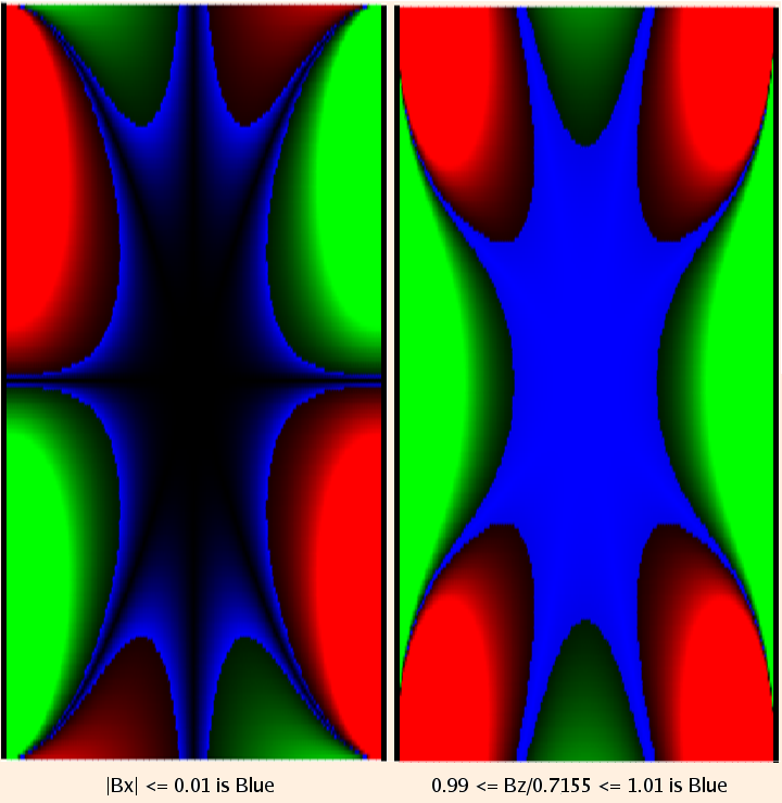
(8 / (5 √ 5) ≈ 0.7155; solid red (above) or green (below) represents 10% deviation from the central value.)
So we see that the Helmholtz Coil can be used to generate an essentially constant magnetic field in a finite region.
These "Amperian loops" are often useful:
B * 2 π r = μ I
B = μ I / (2 π r)
B * 2 π r = μ * n * 2 π r I
B = μ n I
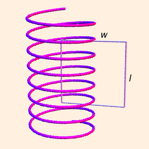
If the Amperian loop is interior to the coil (between the center of the figure and the wires), the enclosed current is zero, and hence so
is B. If the loop is exterior to the coil (beyond the wires), for every current element that crosses the plane of the loop in one direction, there
is an identical current element crossing in the opposite direction, and so B is again 0.
B * l + 0 * w + 0 * l + 0 * w = μ n l I
B = μ n I
It turns out the calculation is virtually identical to the one we did for a linear electric charge, with the same result: for a straight current element
whose ends are 10 times further away than the field point near the center, the error is again 0.5 %.
The Magnetic Field
B = (μ / (4 π)) I ∫ dl ⊗ r / r3,
where (again, for a uniform medium) μ is the magnetic permeability and
μ0 (for a vacuum) ≡ 4 π * 10-7 T m / A. Note that the form of the Biot-Savart law is the same as
Coulomb's law with the substitutions
Note that the direction of integration must be in the direction of current flow.
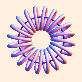
The direction of B can be given by another right hand rule: place the thumb of your right hand along the current; the field
will be tangent to the curved fingers of your right hand. In this figure, the black arrow is the current and the red and blue arrows
show the direction and magnitude of the magnetic field at the base of each arrow:
F = It ∫ dlt ⊗ B
we see that parallel currents attract, and anti-parallel currents repel.
r = (x - s cos θ, y - s sin θ, 0)
Using the same substitution we used for the electrical potential:
= ((y - s sin θ) cos θ - (x - s cos θ) sin θ) k ds
r = √ (s2 + x2 + y2 - 2 s (x cos θ + y sin θ))
u = s - (x cos θ + y sin θ)
we have
= s - a
B(x,y,0) = (μ I (y cos θ - x sin θ) k / (4 π))
∫- ab - a du / (u2 + x2 + y2 - a2)3 / 2
In a similar fashion, we can compute the field due to a current element from (-b,0,0) to (b,0,0) as (note the negative sign required
for the correct current flow)
= (μ I (y cos θ - x sin θ) k / (4 π))
u / ((x2 + y2 - a2) √ (u2 + x2 + y2 - a2)) |- ab - a
(b - (x cos θ + y sin θ)) / √ (b2 + x2 + y2 - 2 b (x cos θ + y sin θ))) /
(y cos θ - x sin θ)
B(x,y,0) | θ=0 - B(x,y,0) | θ=π
which in the limit b → ∞ is
= (μ I k / (4 π y)) ((b - x) / √ ((b - x)2 + y2) + (b + x) /
√ ((b + x)2 + y2))
B = μ I k / (2 π y)
(r cos θ, r sin θ, b * r / 2)
where b = +1 or -1 (we will do each loop separately).
dl = (-r sin θ, r cos θ, 0)
and
dl ⊗ r = (-b/2 r2 cos θ, -b/2 r2 sin θ, r (r - a cos θ)).
Integrating with respect to θ, from 0 to 2π, we obtain (for both loops together) a very complicated function, whose
only nonzero component is in the z direction. But expanding in a Taylor Series about a = 0, we find that the result simplifies greatly, to
B = 8 μ N I / (5 √ 5 r) k + terms of order a3.
If we allow the field point to vary in z as well, the result is even messier, but numerically we can see that Bx and
Bz are constant in a finite region between the coils (By is identically zero since we have computed B
in the x-z plane):
∫closed loop B ⋅ ds = μ I,
where I is the total current passing through the closed loop (imagine the loop as the boundary of a disc; the currents that contribute
pierce the disc, with positive sign if the current is parallel to the normal of the disc as determined by the right hand rule).
For both the toroidal coil and the solenoid, B is strictly constant inside the coil and zero outside only in the ideal limit where the
individual turns of wire can be considered tightly packed circular current loops (and in the case of the solenoid, an infinitely long coil).
A long straight current, field point a distance r from the current, in a plane perpendicular to the current:
 n loops per unit length, field point inside and coaxial to the toroidal coil, a distance r from the center of the figure:
As with Gauss' law, the Amperian loop must intersect the field point. Also, the loop must be far from ends or corners of a real current.
Use the right hand rule to decide the direction of B, and where it is zero and nonzero.
We should also ask the question "how far from the ends is far enough?"
ΦB ≡ ∫ B ⋅ dA.
Because there are no point-like objects with magnetic "charge", Gauss' law gives us
∫closed surface dΦB = 0.
∇ ⋅ A ≡ dAx/dx + dAy/dy + dAz/dz,
and the curl:
∇ ⊗ A ≡ (dAy/dz - dAz/dy, dAz/dx - dAx/dz,
dAx/dy - dAy/dx).
With these definitions,
B = ∇ ⊗ A.
Gauss' law can be written as
∇ ⋅ B = 0,
and is then a result of the identity
∇ ⋅ (∇ ⊗ A) ≡ 0.
| (prev) | (top) | (next) |
©2010, Kenneth R. Koehler. All Rights Reserved. This document may be freely reproduced provided that this copyright notice is included.
Please send comments or suggestions to the author.