The experimental apparatus
All of the limit sets I'll display here were generated in the same fashion:
- The generators are constructed either using their actual components, or from one of the following methods
(I did a fair amount of experimentation to get to this point!):
- using the traces tr(a), tr(b) and tr(ab) (Mumford, Series and Wright):
P = tr(a)2 + tr(b)2 + tr(ab)2 - tr(a)tr(b)tr(ab)
Q = ± √(4-P)
R = ± √P
a = {{tr(a)/2, (R+tr(b)) (iQ*tr(a)+2tr(ab)-tr(a)tr(b)) / (2(tr(b)2-P))}, {(tr(a)2-4) (tr(b)2-P) / (2(tr(b)+R) (iQ*tr(a)+2tr(ab)-tr(a)tr(b))), tr(a)/2}}
b = {{(tr(b)-iQ)/2, (tr(b)+R)/2}, {tr(b)2+Q2-4) / (2(tr(b)+R)), (tr(b)+iQ)/2}}(the sign on R is chosen to avoid singular matrices; the other ± sign is chosen to make all fixed points lie on or in the unit circle, if that is possible)
I worked this out myself following Mumford et. al., and my result is slightly different but is still correct. A careful eye will notice that my limit sets are conjugate reflections of theirs.
Note that this method produces singular matrices when either P=tr(b)2, or P=4 and tr(ab)=tr(a)tr(b)/2.
- using the Maskit parameter μ:
a = {{-iμ/2, i ± μ/2}, {-(μ2+4)/(4i ± 2μ), -iμ/2}}
b = {{1-i, 1}, {1, 1+i}}(where the ± sign is chosen to make all fixed points lie on or in the unit circle; note that with μ=2i and the negative sign choice, a becomes the identity matrix; this corresponds to the (0,1) "gasket", whose limit set was computed using the components
a = {{1, 0}, {-2i, 1}}
Again, this is different from Mumford et. al. There are two solutions to the Markov identity
b = {{1, 1-i}, {1, 1+i}})tr(a)2 + tr(b)2 + tr(ab)2 = tr(a) tr(b) tr(ab)
and I have used the other one. - using the Riley parameter λ:
a = {{1, 2}, {0, 1}}
b = {{1, 0}, {λ, 1}} - using the traces t(b) and t(ab) (assuming a is parabolic):
a = {{1, i}, {0, 1}}
b = {{1, i(tr(b) - 2) / (tr(ab) - tr(b))}, {-i(tr(ab) - tr(b)), tr(b)-1}}(here tr(ab) ≠ tr(b))
- using the traces t(a) and t(b) (assuming the product ab is parabolic):
P = √(4 - tr(a)2)
a = {{(tr(a) ± i P)/2, 0}, {±(P (tr(b)-2) ±i (tr(a) tr(b)-4))/2, (tr(a) - ±i P)/2}}
b = {{1, i}, {i (2 - tr(b)), tr(b)-1}}(the sign choice here is an input)
- using the traces tr(a), tr(b) and tr(ab) (Mumford, Series and Wright):
- After fixing a and b, I then computed A, B and the commutators abAB, AbaB, BabA and ABab, and their inverses.
- If a "special word" (a string of a's and B's which is parabolic) has been input, it and its inverse are computed.
- Each of the generators, commutators and the special word have two fixed points:
z = (g1,1 - g2,2 ± √(tr(g)2-4)) / (2g2,1)
These are computed (the fixed points of their inverses are the same).(gi,j are the matrix components)
- The plot area is a fixed size in pixels; if zmax is the largest absolute value of the fixed points,
the coordinates of the corners are set to ±zmax±i zmax.
Outside of the Maskit slice, zmax varies considerably, and will be specified for those limit sets below.
Whenever a method produces multiple conjugates which yield finite values of zmax, if one of the conjugates yields a zmax of 1, that is chosen; otherwise, the conjugate with the smallest zmax is chosen.
- If zmax is 1, the program randomly iterates left multiplication
by a, b, A and B (but avoids the inverse of the last multiplication, to avoid wasting time), and
after each iteration it maps the unit circle using the resulting product g:
z = 1/(-g2,2/g2,1)*
At this point the plot is a collection of discs which are each equivalent to the exterior of the unit disc; for a cusped group, these discs represent an approximation to one half of the regular set of the group.
center = g.z
radius = |center - g.1|(where "*" indicates complex conjugation and "g.z" indicates
(g1,1z + g1,2)/(g2,1z + g2,2)).
Each new circle (disc) with a radius larger than two pixels and lying within the plot area is colored in light gray (the radius is reduced by two pixels to guard against rounding errors in the auto-detection of non-discrete groups; see step 7). After (by default) 100 iterations (corresponding to a word length of 100), the process starts over.If the program is used interactively, the plots are displayed in real time using OpenGL; if the program is being used in batch mode, to create a png file of the plot, the "circling" stops after a total of one million iterations.
- The iteration process described above is now applied to every fixed point computed in step 4. Each fixed point is
associated with a different color, and once a point is plotted another cannot be plotted there. The maximum word length
here defaults to 200. If the program is generating a png file, the total number of iterations is (by default) eight million.
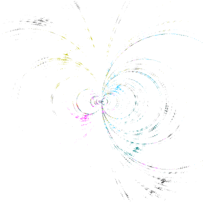
The resulting plot now includes a dust approximation to that portion of the limit set of the group lying within the plot area:
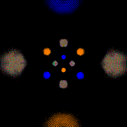
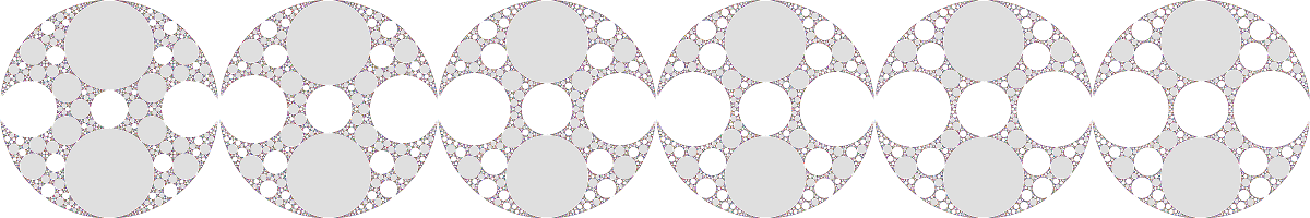
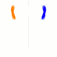
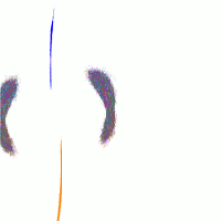
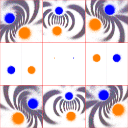
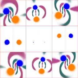
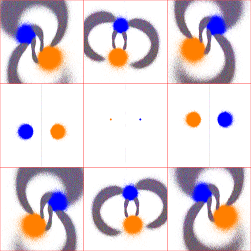
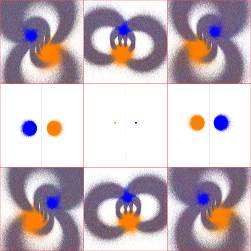
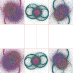
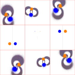
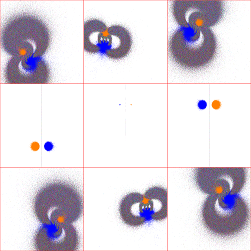
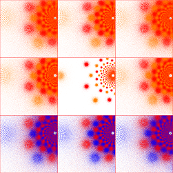
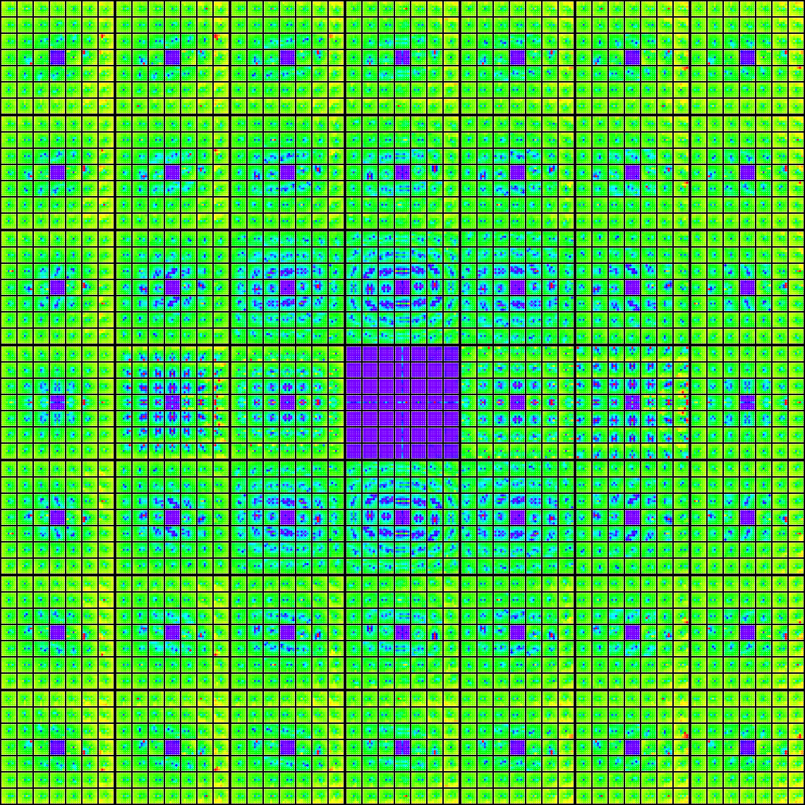
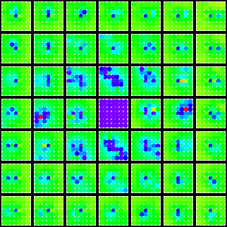
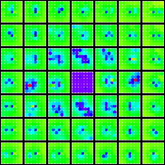
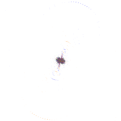
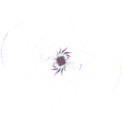
A sample plot (the (2,15) gasket group), and a blow-up of the central region showing the color-coding of the fixed points: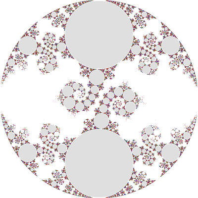 ........
If any limit set point has landed on a previously-mapped circle, the program flags the group as non-discrete.
- Finally, the program outputs the number of points and circles plotted.
Adjustable parameters include the corner coordinates and the maximum word length l (which defaults to 200). If l is modified, the total number of fixed point iterations is set to l3, but the maximum number of circle iterations is left at one million.
The program uses the number of seconds past January 1, 1970 as a seed for the random number generator. Curious about how much variation occurs in the limit sets due to the stochastic nature of the algorithm, I created limits sets for the (2,5) gasket group (see below) about five days apart. The two limit sets were identical. For these plots, the plot area was 800 pixels2. Wondering whether increasing the plot size would alter the situation, I ran two more with a plot area of 3200 pixels2, a few minutes apart. Again, the results were identical.While all of the limit set plots were done in this fashion, the Riemann surface plots, the real trace rays and all color contour plots were done using Mathematica 7.0. Gimp was used to pinch curves on the Riemann surfaces, and ImageMagick was used to build the montages. LibreOffice was used for simple data analysis.
All computations were done in double precision. Because this work is based on numerical computation, it is important to know what hardware was used. These calculations were done on two Intel Core Duo CPUs, an E8400 stepping level 10, microcode level A07, and an E7500 stepping level 10, microcode level A0B. These processors use 64-bit doubles, with 52 bits for the significand, giving more than 15 digits of precision; in both, computations in the CPU use 80-bit doubles with 64 bits for the significand, giving more than 19 digits of precision. Both OS are Slackware 14.2, running kernels 4.14.11 or later (kernel and library upgrades occurred on the E8500 during the course of this work). The program was compiled with gcc -Wall -Wconversion -g -Og, which is supposed to optimize while facilitating debugging (some variables were optimized out).
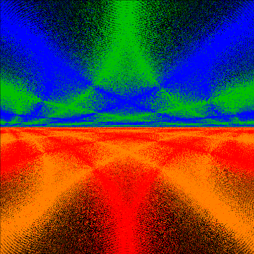
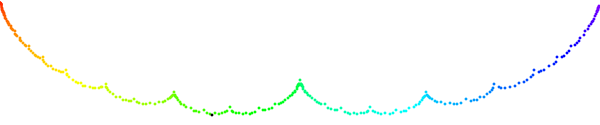
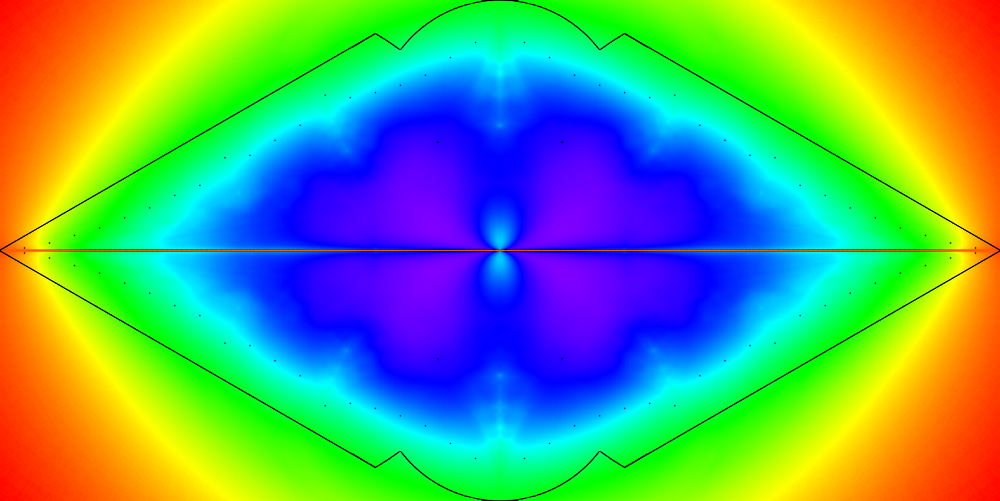
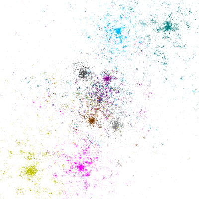
While working on this project I made an interesting observation, based on plots like these:
(tr(b) varies from i at bottom left to 8+9i at top right)
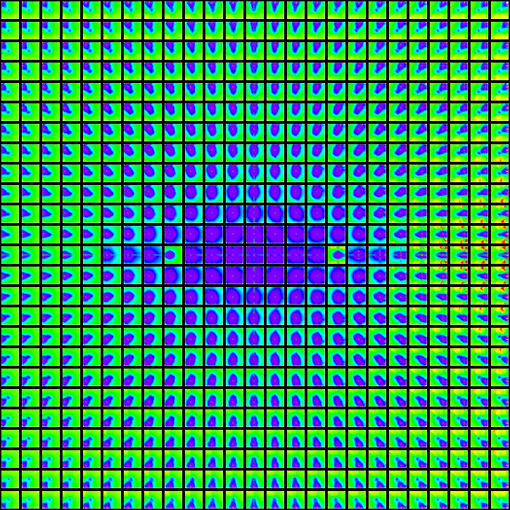
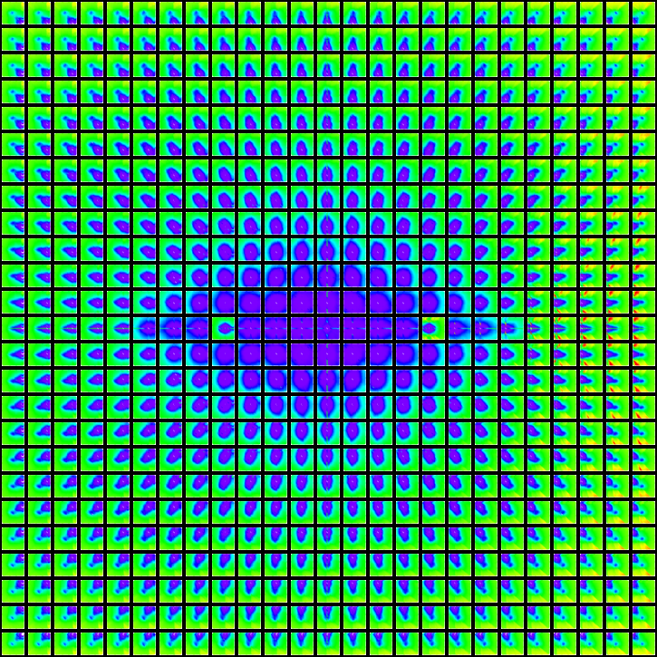
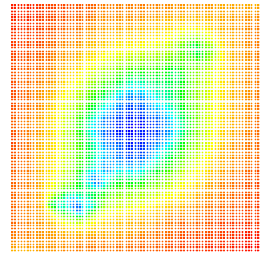
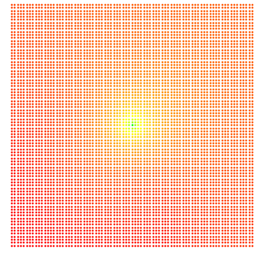
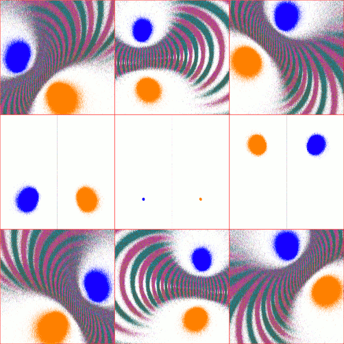
- The first plot shows which groups were nondiscrete, based on simple visual analysis of over 6,000 limit plots.
- The second plot encodes the Log10 of the number of points displayed in each limit plot I created for those traces, with Nmin = 93 encoded as red (outer edges), and Nmax = 948,747 encoded as magenta (center).
- The third plot shows Log10(zmax) for those traces, with zmax ranging from 1.131 (red) to 1768.21 (magenta).
The point density closely mirrors the discreteness of the corresponding groups, although it hides what I suspect is a fractal boundary for the non-discrete groups (based on what we'll see below in the Maskit and Riley slices). The zmax plot clearly indicates the center of the non-discrete region, but it is clear that zmax drops off quickly as distance from the value of tr(ab). I've used the point density visualization technique in all of the sectors of Teichmuller space that I have investigated. The plots were made using Mathematica. To standardize the plots, all of the limit sets used to do this had fixed word length=100, iteration limit=106 and zmax=1.
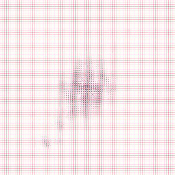
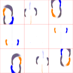
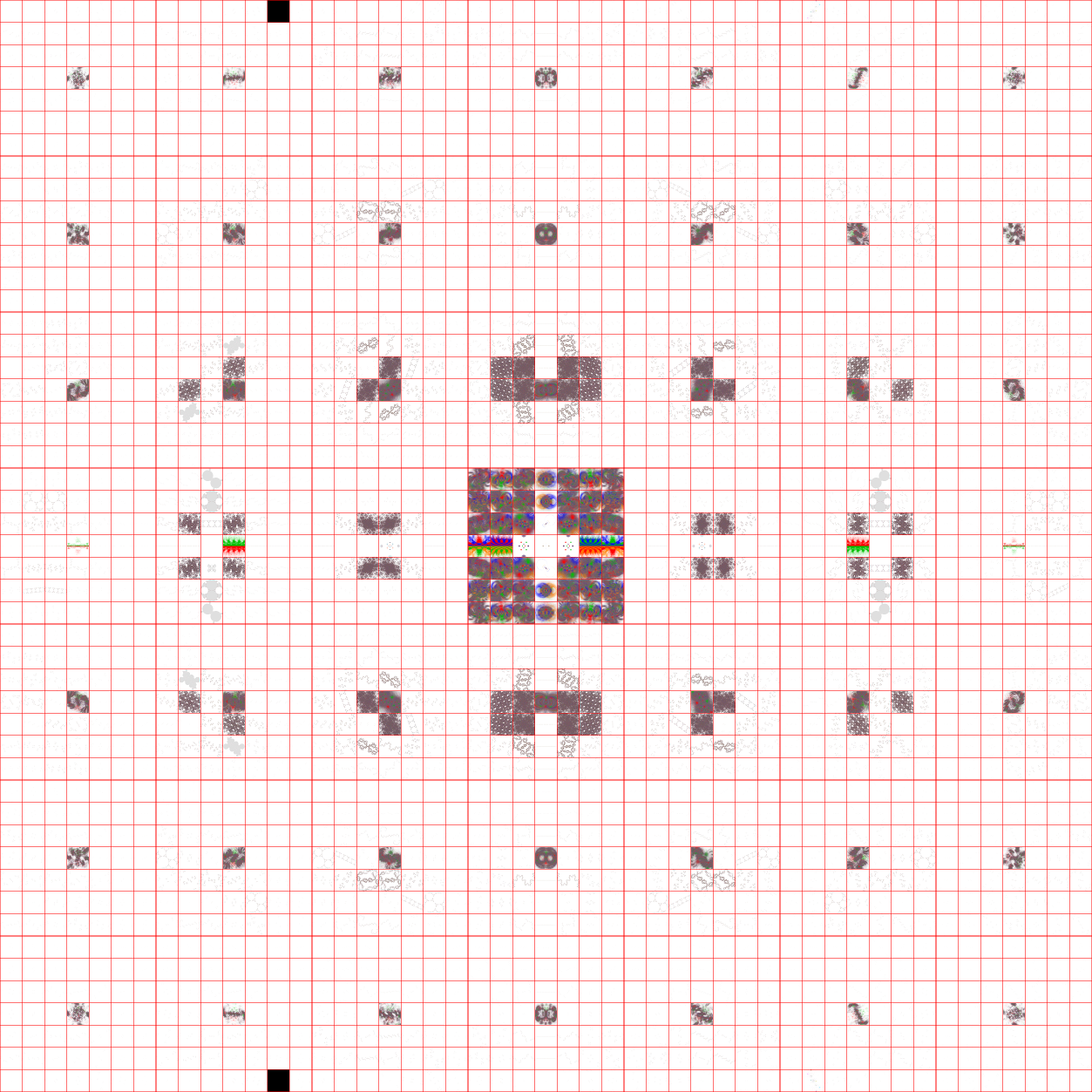
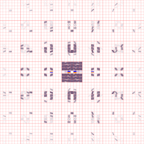
Teichmuller space is a manifold with boundaries, so locally it is homeomorphic to Rn (n is discussed below). Sampling is therefore required in any study of individual limit sets. In order to make the first plot of the three above, I had to plot 6,561 limit sets. These were sampled at intervals of 0.1 and 0.1i. But in general it is unclear whether this, or any particular, level of detail is sufficient to display the nature of any finite region of the space. In order to get a feel for this, I looked at the same region, but with the more course intervals of 0.5 and 0.5i. These two plots have been scaled to the same image resolution for comparison:
 ........
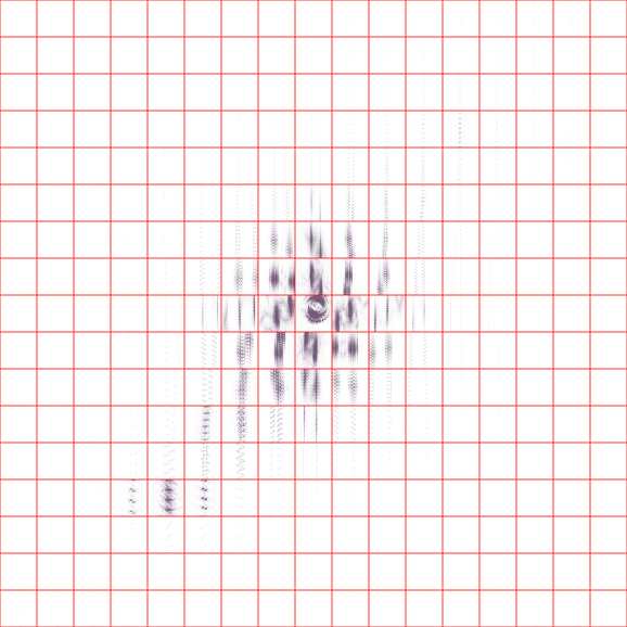
Modulo isolated instances, the limit sets appear to be "continuous functions" of their coordinates in Teichmuller space. Because of the large number of limit sets involved, in most cases I have opted to sample at intervals of 1 and i.
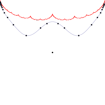
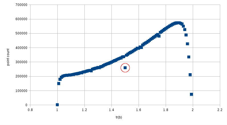
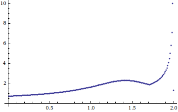
Since we will be plotting hundreds of thousands of limit sets, some discussion of performance is warranted. When running the program interactively, the user is responsible for deciding when to terminate the algorithm. Whether mapping circles or fixed points, it is usually clear that after a short while the time between "new" points (circles) becomes very long. When running the program in batch mode, the program as described arbitrarily terminates after l3 iterations, where l is the word length. The following plot describes the results of plotting the (2,5) gasket for word lengths varying from 100 to 1000:
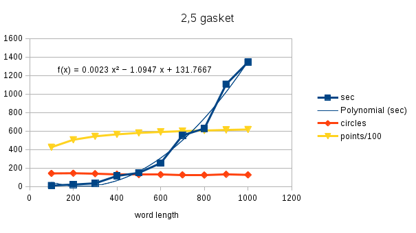
The time required to complete l3 iterations increases approximately quadratically with l. For all this effort there is essentially no improvement in the number of circle maps, and little improvement in the number of fixed points mapped after l=400.
Wanting to investigate longer word lengths, I modified the program as follows:
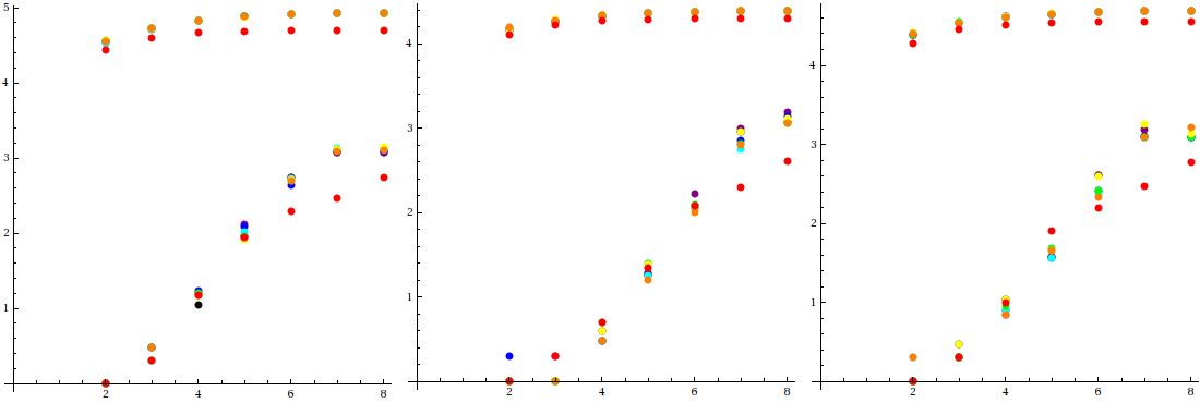
I then ran a number of tests, with the word length varying between ten and 3,200, and maxit varying from 100 to 100 million.
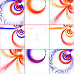
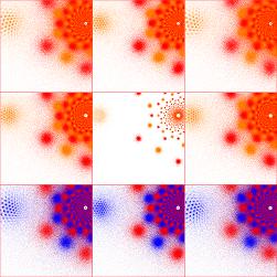
The first tests were for the (2,5) gasket (left), and the gaskets at μ=1+2i (middle) and μ=1+√3i (right):
Horizontal axis is log10maxit; lower plot is log10runtime(s), upper plot is log10points;
color varies with word length according to the following key:
With the original termination criteria and a word length of 200 (which implied an iteration limit of 8 million), the (2,5)
gasket took 21 seconds and generated 50,538 points. With the new criteria, a word length of 200, and maxit set to 1,000, the plot
completed in 2 seconds and contained 53,179 points. While there was little improvement in the point tally for word lengths above 200,
it is worth noting that a word length of 3,200 and a maxit value of 10,000 generated 65,985 points in 10 seconds.
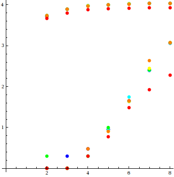
I also ran tests for the quasifuchsian group for tr(a)=-2-i, tr(b)=-3-i (right; word length = 3,200, maxit = 10,000):
Looking at the data, it seems that there is little need to consider word lengths above 50, or maxit values above 10,000.
While larger word lengths and maxit values seem to yield higher point counts, the difference is hardly worth the processing time.
Any complete hyperbolic 3-manifold M is the quotient of H3 by a Kleinian group G, with fundamental group
π1(M) isomorphic to G.
Its limit set Λ(G) (of all fixed points of G) lies on the S2 at ∞
(which is taken to be the "boundary" of H3, and is isomorphic to E2).
The complement of Λ(G) in E2 is Ω(G), the regular set.
Teichmuller space is the quotient of the space of metrics admissible to R by the action of diffeomorphisms
homotopic to the identity, by a homotopy which takes the boundary into itself at all times.
(Thurston, section 4.6)
There is therefore not a 1:1 correspondence between points in Teichmuller space and the space of all hyperbolic manifolds; conjugate
groups g and g' (where g'=hgH for some h in Moeb(E2)) describe the same manifold. When the program
chooses a ± sign, it is actually choosing between conjugate groups. For the hyperbolic, quasifuchsian and cusped groups below,
there are two limit set plots, one for each sign choice. For the other limit sets, I include one which has been conjugated by
It should now be clear why I have restricted myself to the genus 2 case: the corresponding Teichmuller space has complex
dimension 3. This makes it impossible for creatures like myself, inhabiting a world with 3 real spatial dimensions, to visualize
any Teichmuller space. As we will see, at best one can look at cross-sections, and try to imagine how they fit
together.
I'm also very interested in Moebius subgroups which do not generate hyperbolic manifolds. These groups are non-discrete;
an infinite sequence of group operations converges to the identity, and the limit set is the entire complex plane.
If you can characterize the transition from discreteness to non-discreteness, you can identify a boundary in Teichmuller space.
Another interesting type of Moebius subgroup is the non-free group. Here, a finite sequence of group operations equals the identity
(which of course means there the group contains elliptic elements). In this case, the limit set is a set of isolated points (dust),
and the quotient Ω(G)/G is an orbifold. Non-free groups seem to be isolated points in the larger space in which Teichmuller
space can be embedded.
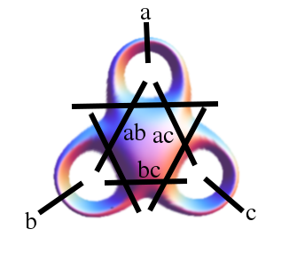
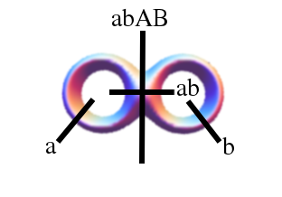
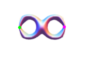
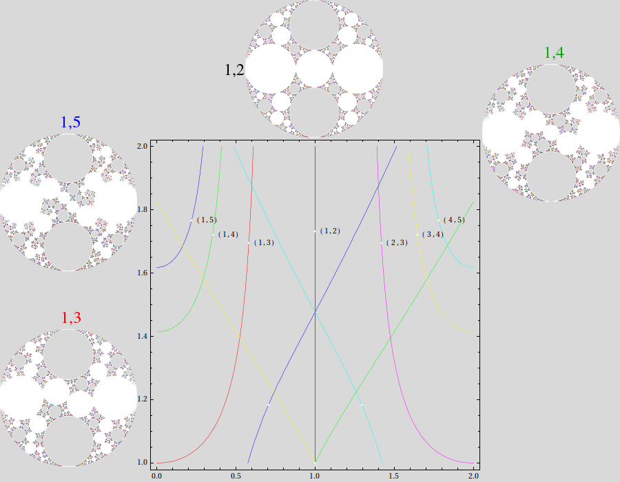
I'll now specialize to genus 2. The two-holed torus can be pinched in four ways:
(method 3 (λ = 0.05+0.93i), tr(ab) = 2.1+1.86i;
(method 2; μ = 0.766588417465459-1.642138768653476i);
The purely-hyperbolic groups constitute the vast majority of Teichmuller space; the other cases are, after all, special cases.
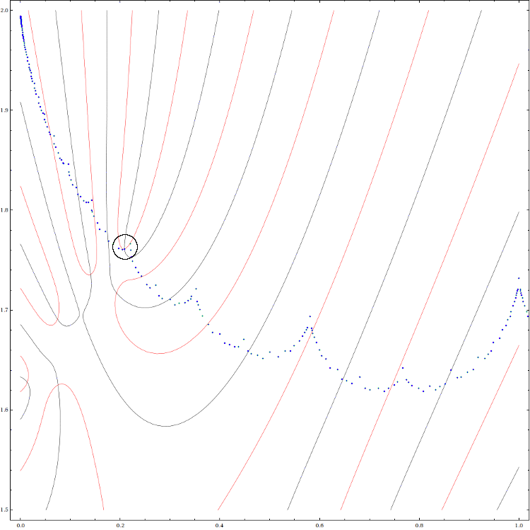
Let's examine the special cases in more detail, starting with the most constrained:
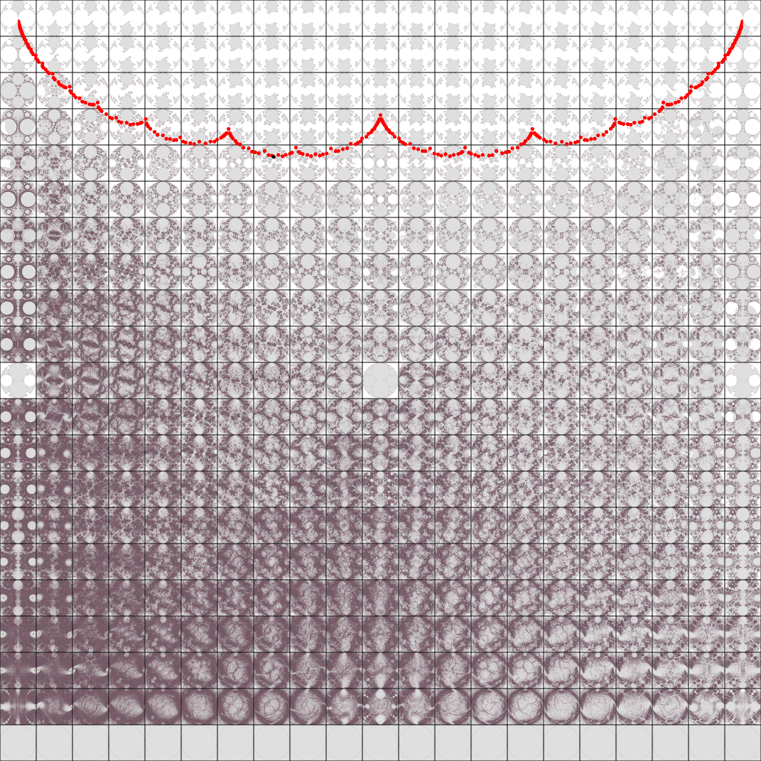
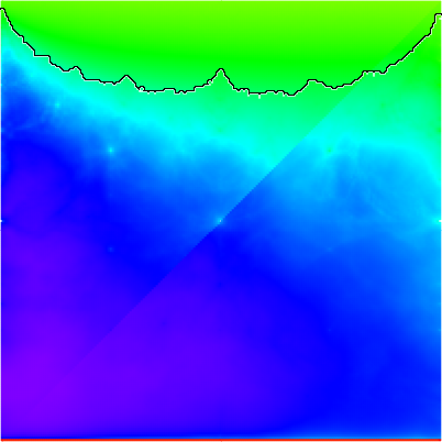
(zmax = 1 for all Maskit slice limit sets)
The red points trace the Maskit boundary; all groups on the boundary are gaskets (doubly-cusped, with a special word of trace 2)
or degenerate (the black point marks a degenerate group), and
all groups above the boundary are discrete and singly-cusped. All groups below the boundary are either non-discrete or
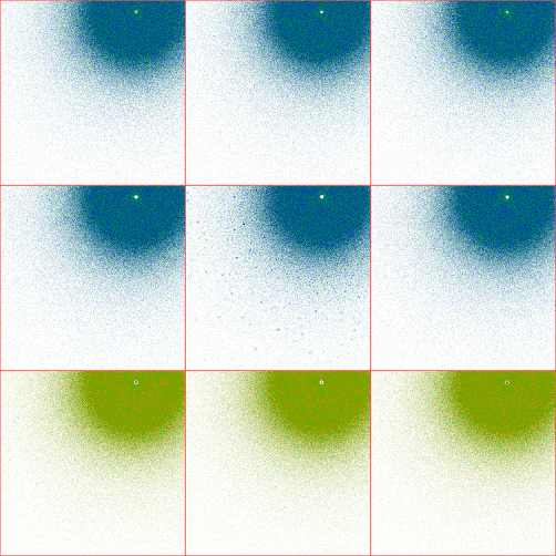
non-free; examples of the latter are at μ=i, and of course μ=2+i.
The samples with im(μ)=0 (at the bottom), whose limit sets are a circle, appear to have the two sides of the regular set
identified (μ=0 is a non-free group; tr(a)=0, so a2 is the identity matrix).
This also seems to be the case for the (1,4) gasket group at μ=1+i.
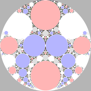
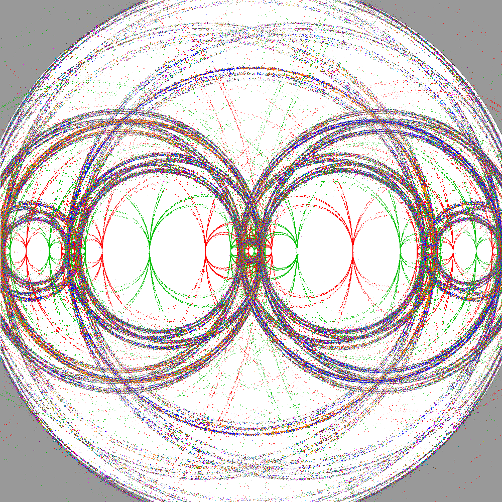
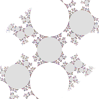
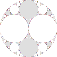
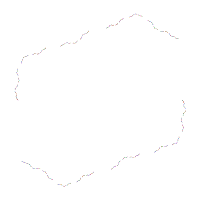
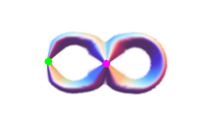
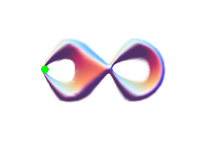
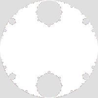
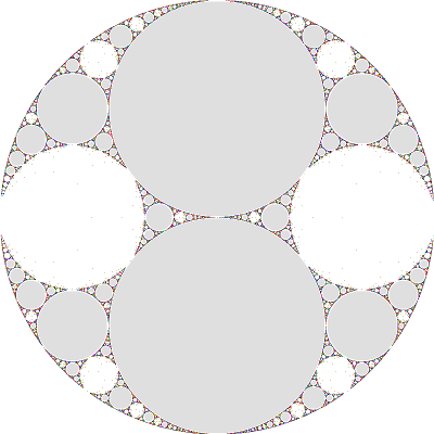
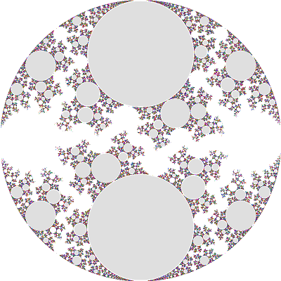
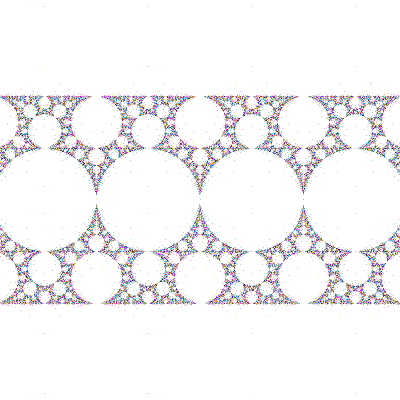
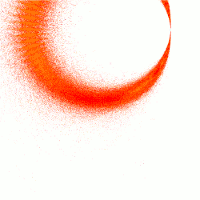
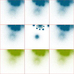
The limit sets in the upper two corners (μ=2i and μ=2+2i) are the Apollonian gasket (here shown with one
of its conjugates):
It is the prototype for the doubly-cusped groups.
The gasket groups are identified by the integer number of twists on the "a" and "b" punctures, designated q and p, respectively.
The Apollonian gasket is the (0,1) group. In principle, one can find all of the (p,q) groups as follows (following
Mumford et. al.):
(Nmin = 2,590, Nmax = 550,550)
The slice was sampled at intervals of 0.01 and 0.01i. All groups sampled below the black line were auto-detected as
non-discrete. The "light spots" indicate non-free groups; the red line at the bottom corresponds to the "identified" groups
on the real axis described above. The plot is markedly non-symmetric about the line Re(μ)=1 because of the tendency for
groups with higher p/q to "fill" more slowly with the stochastic algorithm.
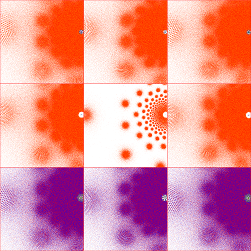
To understand the transition from discrete single-cusp groups to gasket group to non-discrete groups, I plotted an
11-image sequence for Re(μ)=1 and Im(μ)=4, 3.5, 3, 2.5, 2, 1.9, 1.8, 1.732050807568877 (the double-cusp), 1.7, 1.6 and 1.5,
where the last three are non-discrete (μ=1+1.7i is the second plot; click on this image and the sequence will appear in a
new tab):
You can see that the non-discreteness displays itself as an increasing "overlap" between the upper and lower halves of the limit set.
Some of the groups just below the Maskit boundary are very slow to show this overlap. This is probably a function of the limited
resolution of the plots. Of the 3,146 groups examined (step 5 above),
( (2,3) is conjugate to (1,3), (3,4) is conjugate to (1,4) and (4,5) is conjugate to (1,5) )
Gasket groups on the boundary are marked by white dots. The trace polynomials for (1,q≤5) are:
 ........
The structure of Teichmuller space for genus 2
Before concentrating on genus 2, let me review how I got here from hyperbolic manifolds.
A Kleinian group is a discrete torsion-free group of isometries of H3
(and is therefore a discrete subgroup of Moeb(E2)),
which acts properly discontinuously (the inverse image of any compact set is also compact).
The latter implies that a discrete group has a countable number of elements. Kleinian groups are usually
taken to be non-elementary - they leave an infinite number of fixed points on the sphere at ∞ (dim(Λ) > 0).
The components of Λ are either topologically circles, fractal sets, or totally disconnected (every component is a point).
If G has n generators and no parabolic elements, Λ(G) is
totally disconnected, and the boundary ∂M(G) = Ω(G)/G is a Riemann surface R of genus n.
Such a surface has 3n-3 disjoint, non-parallel simple closed geodesics (which divide ∂M(G) into 2n-2 pairs of pants).
The surface can be cut along any such loop and reconnected with a twist.
The Teichmuller space of M, which describes the set of hyperbolic structures on M, can be parameterized by the lengths and twist
angles of each loop.
It therefore has real dimension 6n-6; since it possesses a complex structure, we often say it has complex dimension 3n-3.
(Marden, sections 2.2-2.5)
Specifying that G is torsion-free means G has no elliptic elements (if G has elliptic elements, M is an orbifold,
with conical punctures).
(Thurston Notes, section 5.3)
If G contains parabolic elements, it can have at most 3n-3, and for each parabolic element, the corresponding loop is
pinched to zero length.
h = {{i, -1}, {1, -i}}/√2
which moves the points at ±∞ to (0,i) and the origin to (0,-i).
Since there can be at most three pinches for genus 2, it is clear that in general, there are more ways to pinch a torus than
can be "used" to create hyperbolic manifolds.
The surface R (and hence the corresponding hyperbolic manifold) can be parameterized by three complex
numbers. I will take them to be tr(a), tr(b) and either tr(ab) or tr(abAB). Which ones are specified determine which "sector" of
Teichmuller space they describe:
Note that we do not consider "b" parabolic as a separate case; exchanging generators results in a conjugation.
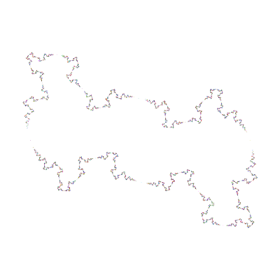
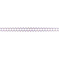
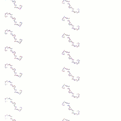
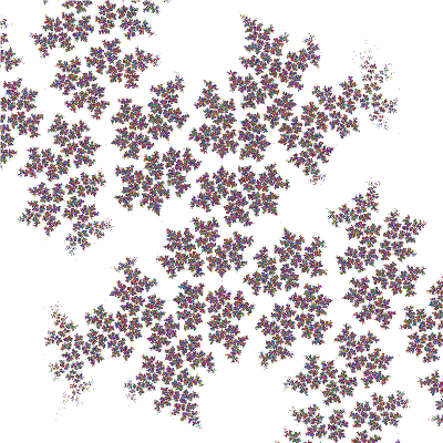
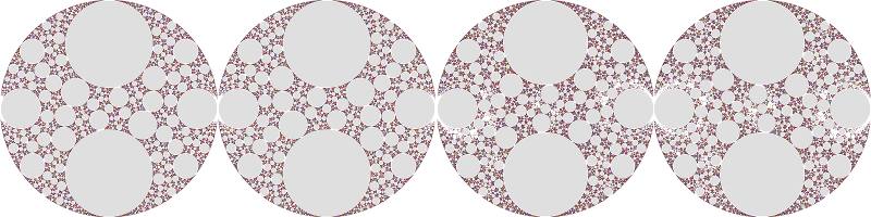
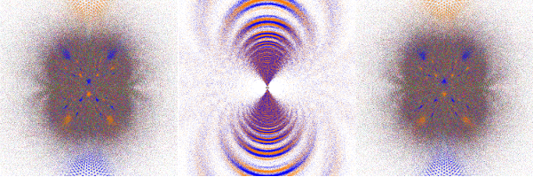
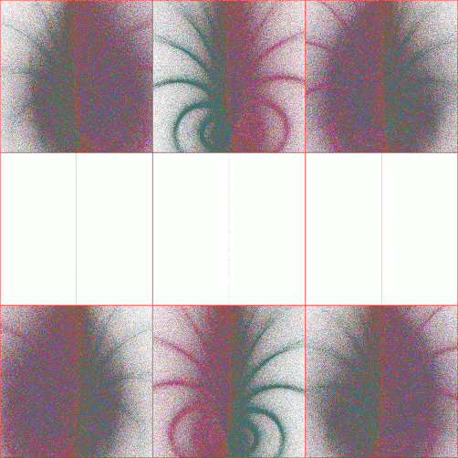
Note the recurring patterns in the limit sets, indicative of translational symmetry caused by a fixed point at ∞.
All limit sets, with any pinching, may be conjugated to a similar form.
Considering what we just mentioned about conjugation, it would seem that while exchanging a and b would not produce a
different hyperbolic manifold, it would describe a different region of Teichmuller space. However, a and b are simply
labels; one does not expect Teichmuller space to care about generator labels.
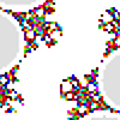
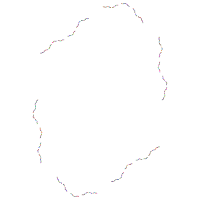
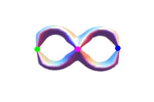
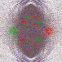
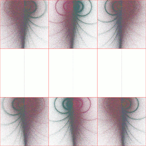
These and the previous pair of limit sets appear to include closed circles. This is an artifact arising from both
the stochastic nature of the algorithm and the resolution of the images. Quasicircles only appear in limit sets when R
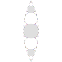
separates into two components ("connected" by a pinch). In genus 2, this only occurs when abAB is parabolic.
G is called a quasifuchsian group.
In each case where a single curve is pinched, we have reduced the problem of "seeing" Teichmuller space to that of a 4-dimensional
space; still difficult, but perhaps approachable.
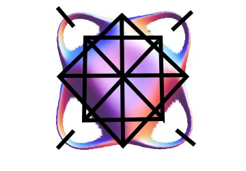
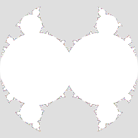
zmax = 1.913 (left), 2.81 (right),
both here multiplied by 12 to get a larger perspective)
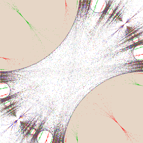
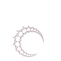
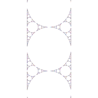
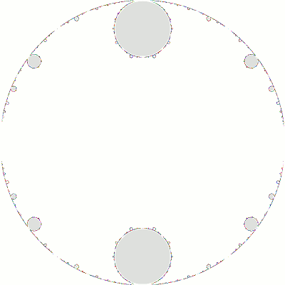
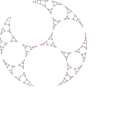
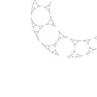
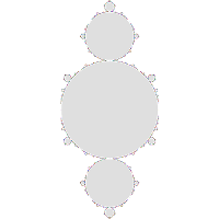
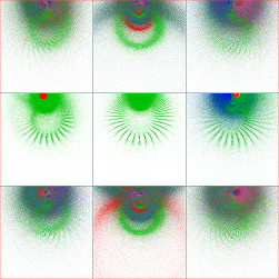
With single-cusp groups, one half of the regular set has closed up into a set of tangent discs, all of which are identified;
the other half is simply connected.
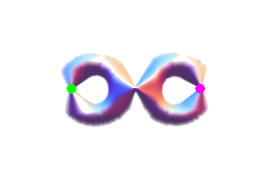
this image corresponds to the (2,5) group, where in addition to b and abAB,
the special word a3Ba2B is also parabolic;
this means the group is doubly-cusped;
the "a" puncture represents a pinch with five complete twists around the "a" meridian, and two full twists around the "b" meridian;
zmax = 1 (left), 3.882 (right))The Maskit slice
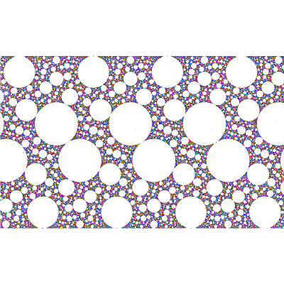
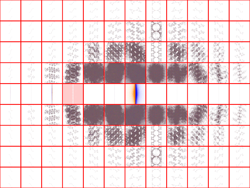
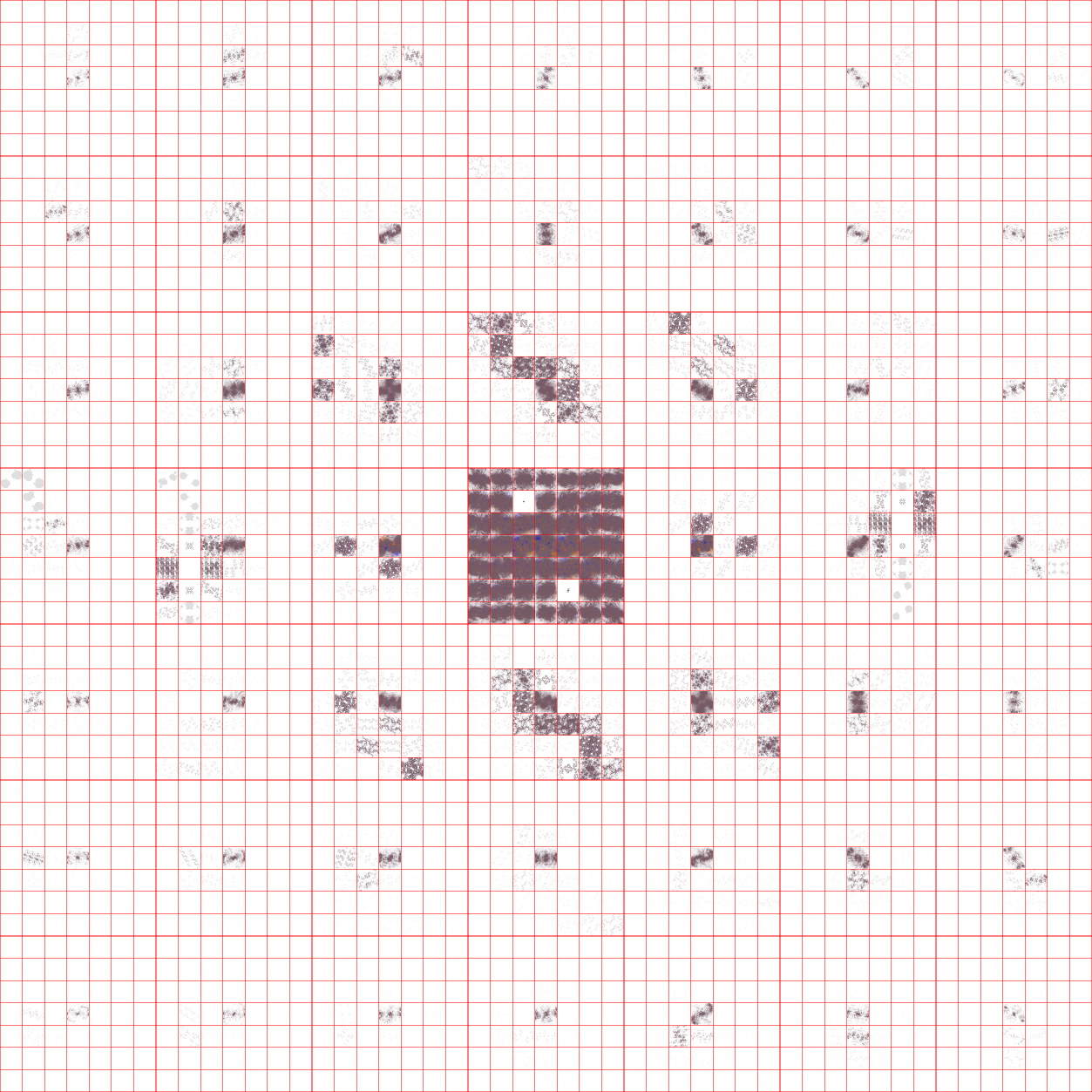
Using the Maskit parameter μ and method 2 above,
Each group G(μ) is uniquely determined by μ, but G(μ) is conjugate to
So we only need focus on im(μ) ≥ 0. For im(μ) ≥ 2, all G(μ) are free and singly-cusped, so our primary region of
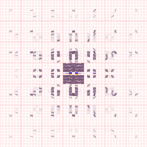
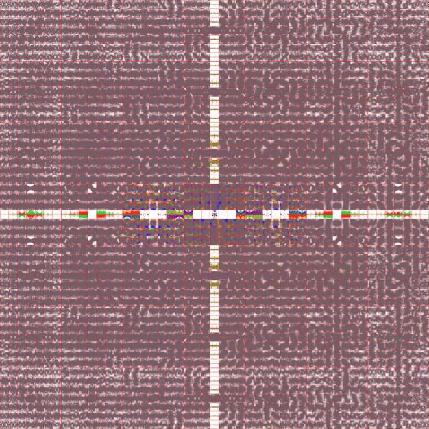
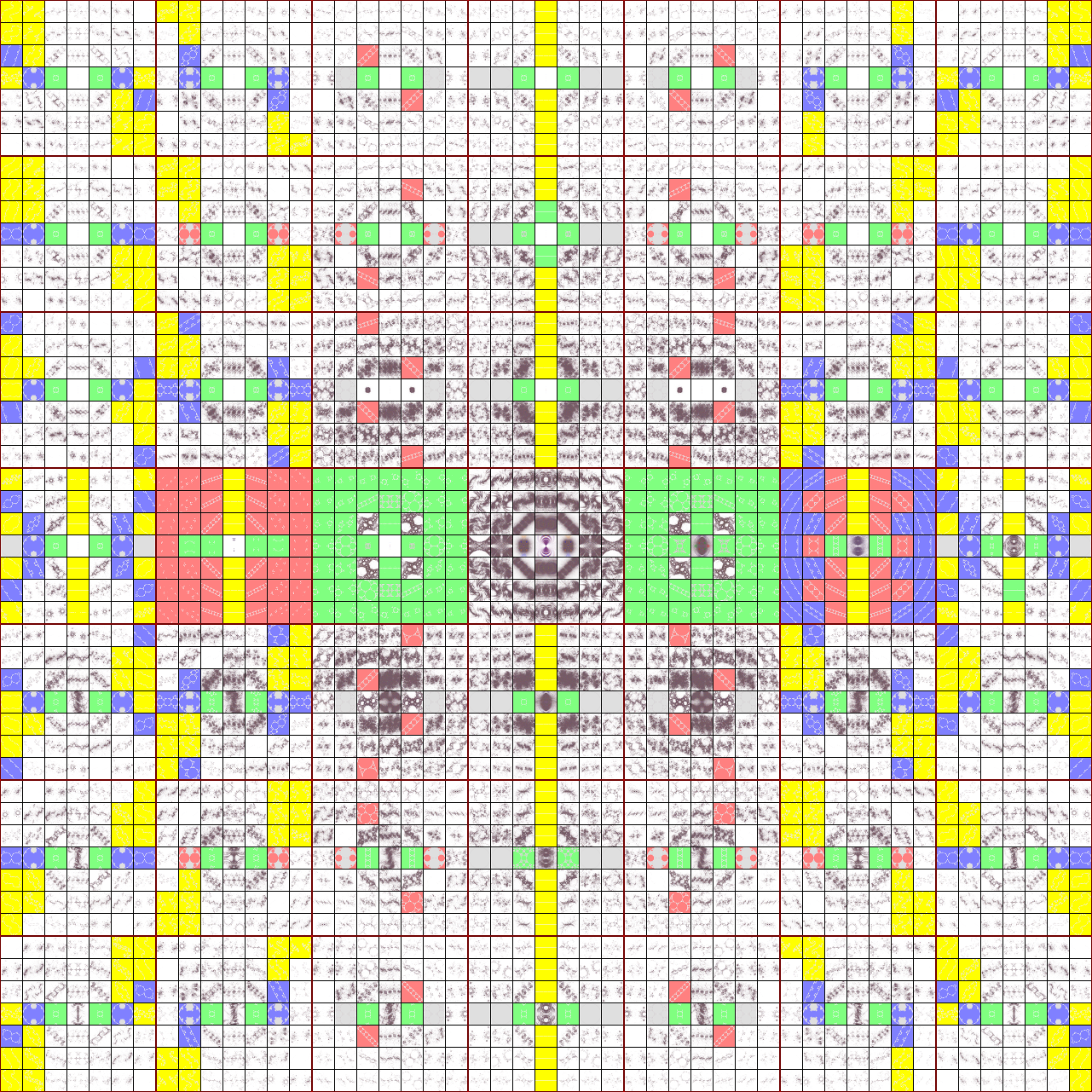
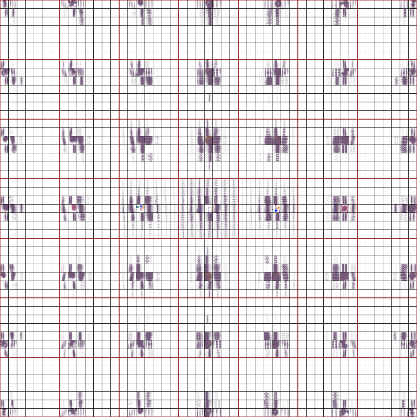
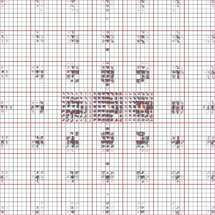
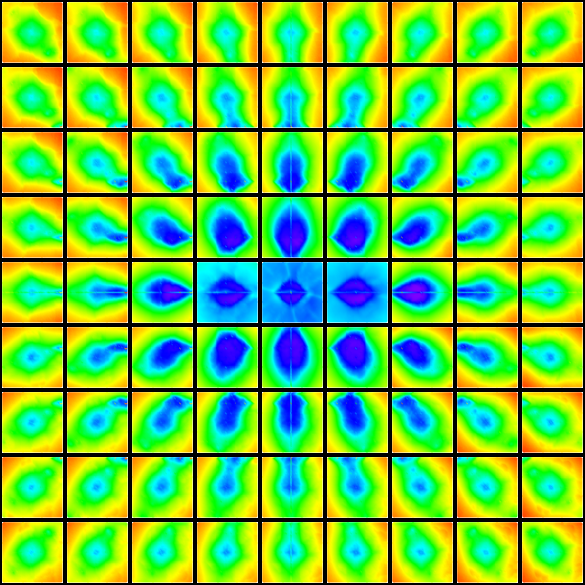
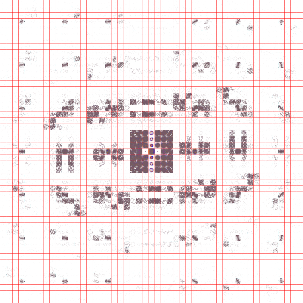
interest is 0 ≤ re(μ) ≤ 2 and 0 ≤ im(μ) ≤ 2. In the montage below, we have sampled this region in increments of 0.1
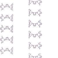
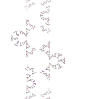
and 0.1i; each sample limit set is centered on its coordinate:
Since the only discrete groups with a geometric meaning are above or on the boundary, groups below the boundary
are not part of the Teichmuller space for the genus 2 torus.
 ........
The majority of the groups shown in the sample plot above are non-discrete; in principle, they should all be completely
colored in. The stochastic algorithm I used to produce all of these limit set plots will only hit all of the points
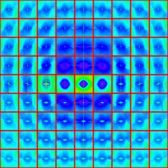
in the complex plane if it is run for an infinite amount of time. The point density plot for the Maskit slice is:
{1, 6, 4, 2, 7, 5, 3, 1}
and the corresponding group word is aaaBaaB.
a = {{-iμ, -i}, {-i, 0}}
find the trace of the special word. For our example, the (2,5) group, the trace is
b = {{1, 2}, {0, 1}}
-i (μ5 - 4μ4 + 9μ3 - 12μ2 + 9μ - 4)
0.375189 + 1.30024i, 1.06548 + 1.2824i and 0.766588 + 1.64214i.
I used Mathematica for this.
For any (p,q), only one solution of the trace polynomial will be discrete and lie on the boundary.
(Mumford et. al.)
w(p+q),(r+s) = w(p,q)w(r,s).
So, for example, w(-1,2) = w(-1,1)w(0,1) = aba.
(This construction works for positive p and q as well.)
(p,q) and (-p,-q) will produce the same word.
Of the 288 limit sets which were not clearly identifiable by the program with word length 1000, 180 were non-discrete
(having stared at over three thousand limit sets by this point, the last few hundred were easily separated by a trained eye).
The (9,20) gasket, which we will look at in more detail below, has a non-discrete solution to its trace polynomial at
μ=0.972815685123106+1.64763216820249i. It is one of the groups which required a word limit of 400 to be auto-detected
as a non-discrete group by the program. In those runs, the plot resolution was 800 pixels2. When the resolution was increased
to 3200 pixels2, the same group was auto-detected with a word length of 200. (At a resolution of 1000 pixels2,
the (6,31) group at μ=0.178840219946299+1.74888845124066i failed to auto-detect non-discreteness at a word length of
102,400 and a maxit value of 108.)
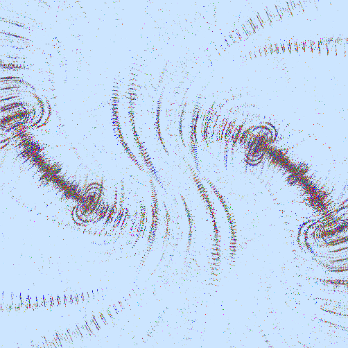
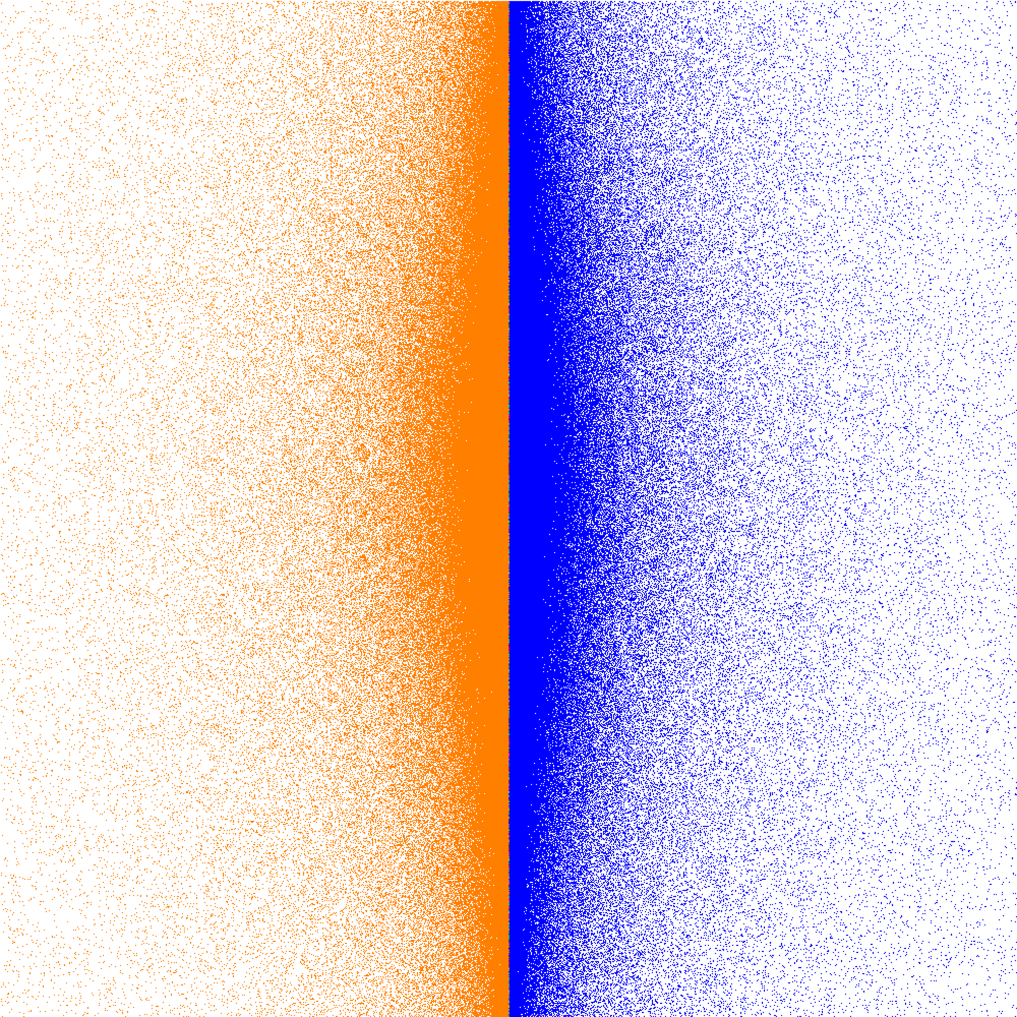
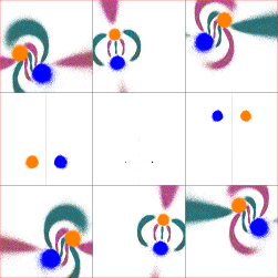
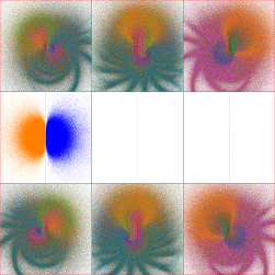
This "overlapping" appears to be ubiquitous; the following sequence for tr(a)=2, tr(ab)=4+5i shows the transition from
tr(b)=4.5+3.5i to 4.5+4i (click for a 6-image sequence):
As part of these computations I have of course constructed trace polynomials P(p,q)(μ) for those 3,146
groups. For any such polynomial, the solution of
Im(P(p,q)(μ)) = 0
is a real trace ray: along that curve the trace of the polynomial is real. Keen and Series
showed that traveling along those rays
from above the Maskit boundary to the point P(p,q)(μ)=2 defining the (p,q) gasket group corresponds to shrinking
the length of the "pinching curve" to zero. Here I have plotted real trace rays for the first few free gasket groups after (0,1):
While the other groups are conjugates, their trace polynomials are different:
Note that the real trace rays for the (1,4) and (its conjugate) (3,4) meet at μ=1+i, the location of the (1,4) group
discussed below.
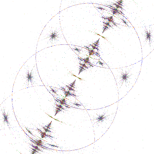
The "landscape" around the (1,3) gasket group is shown below:


(White point at right is the location of conjugate (2,3) gasket group.)
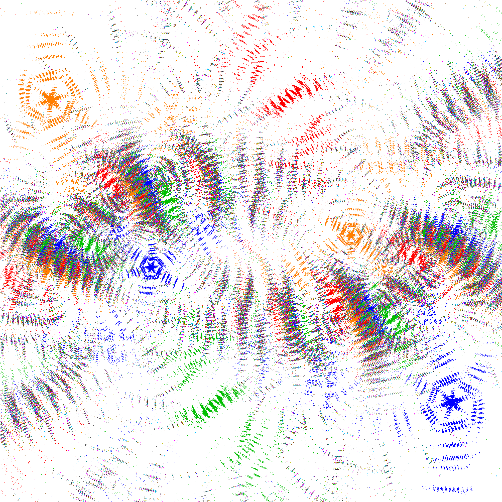
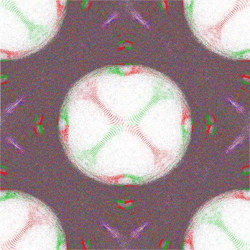
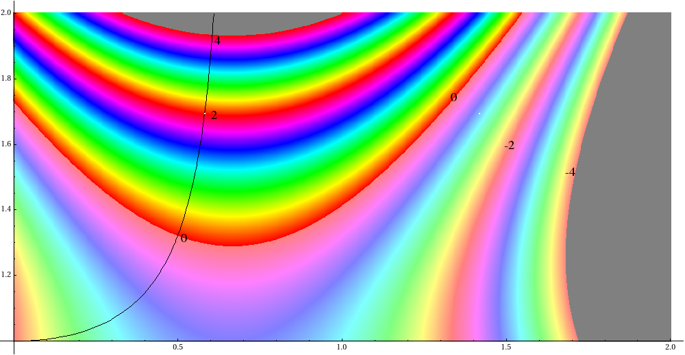
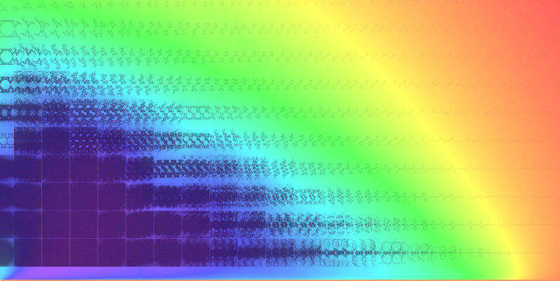
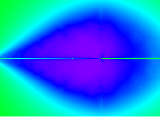
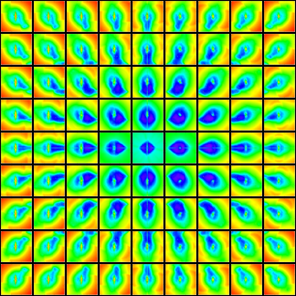
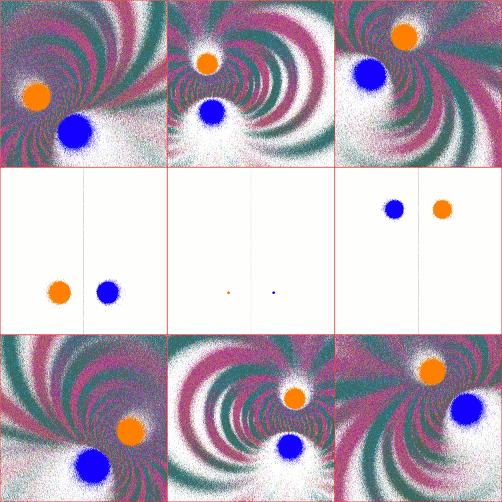
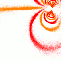
The colors represent Re(P(p,q)(μ)) for values between ±4. Keen and Series were not interested in the analytic continuation of the real trace rays to values < 2 as they appear to have no geometric significance. For a more complicated group, the landscape is much more interesting:
(White points indicate solutions of P(9,20)(μ) = ±2; color contours are as above, with additional -2 contours indicated.)
Keen and Series showed that the real trace rays above the Maskit boundary (for the groups on the boundary) foliate the space above the boundary. The above plot indicates that this will be far from true for the analytic continuations, although the significance of these is unclear.
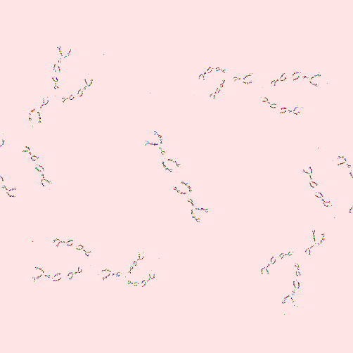
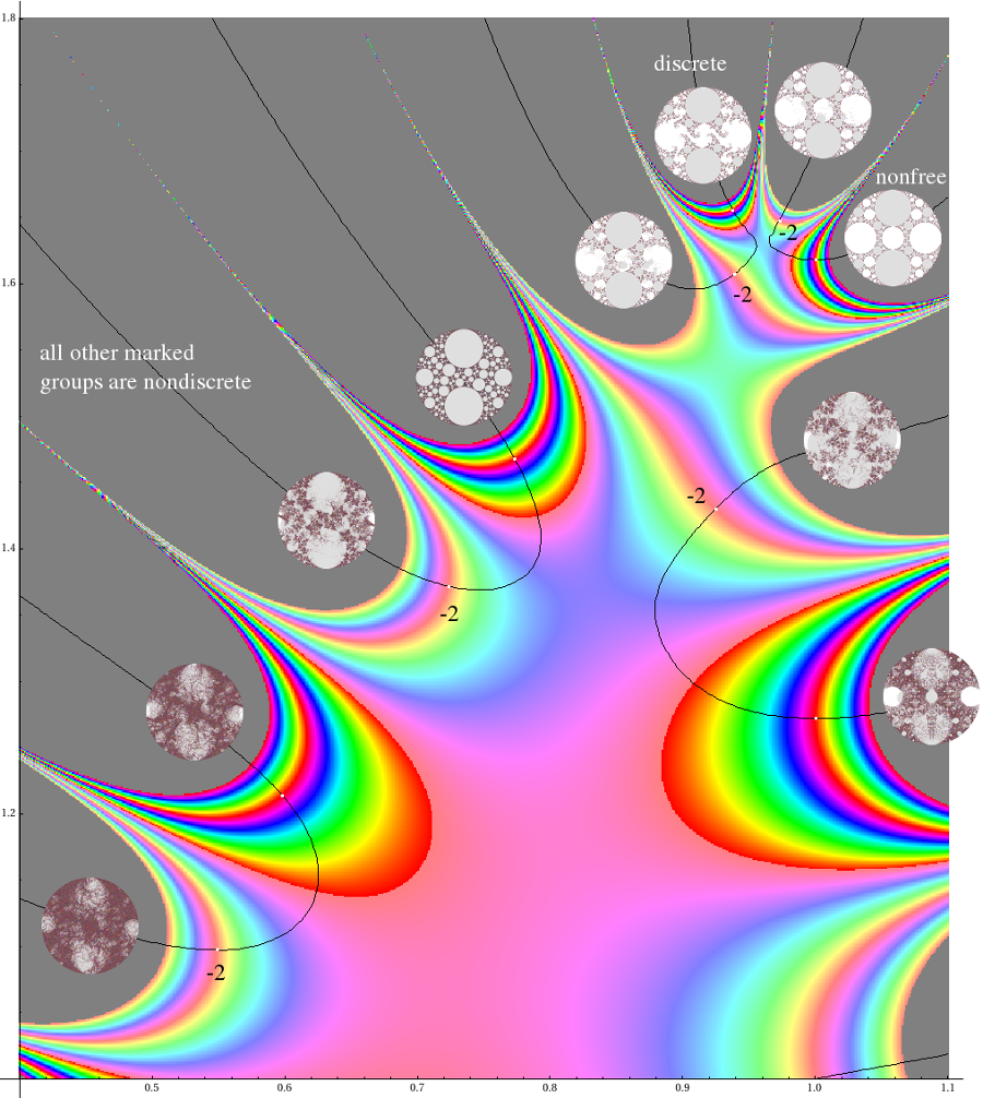
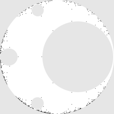
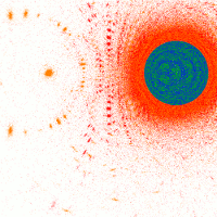
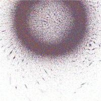
Only at the end, after Amazon had the book and I was playing with gaskets, did I find what seems to be a fool-proof method of identifying double cusps on the Maskit boundary (although I should have seen it sooner!). Here you see a contour plot of the real trace rays of (6,31) (in black) and the solutions of Re(Tr(P6,31)) ≡ 2 (in red) (overlayed with previously identified cusps in blue):As I mentioned previously, (0,k>2) groups are non-free. The (0,3) group is prototypical of these; the image on the right is a blow-up of the large white disc on the right, with circular patterns in the dust emphasized:
Using Mathematica to identify the coordinates of a point close to the intersection of the contours near the boundary (circled), I then used that as a seed to the function FindRoot:
to obtain the value of μ at the cusp: 0.209055933120134 + 1.76110014954012i.FindRoot[{retreq == 0, repolyeq == 2}, {x, 0.213}, {y, 1.765}, WorkingPrecision -> 15, MaxIterations -> 1000]Of course, with Mathematica, the real effort goes into computing the trace polynomial, which in this case is a polynomial of degree 31.
 ........
(μ = i)
Of the groups I've investigated, (p odd and ≥ 5, q=2p+2) all seem to be non-free, although (up to word length 12,800 and maxit value 108) they do not manifest the circular dust patterns:
(from left, (5,12), (7,16), (9,20), (11,24), (13,28) and (15,32); for all, re(μ) = 1;
from left, im(μ) = √2,
1.553773974030037, 1.618033988749895, 1.652891650281069, 1.673898962244985 and 1.687530463435423)
The "rational" points on the Maskit boundary can be labeled by (p,q), with p/q increasing monotonically from left to right:
(p/q ranges from 0 (red) to 21/22 (magenta) for the groups investigated)
But the boundary is continuous, and is indeed fractal.
The "irrational" points on the boundary label degenerate groups, in which one or both sides of the regular set are
empty (for example, the black point above). That territory is replaced by points in the limit set:
(μ = 0.7056734968-1.6168866453i, and tr(a) = 1.5-√(3)/2i, tr(b) = 1.5+√(3)/2i, tr(abAB) = 2 (zmax = 3.732);
If p and q correspond to winding numbers for the twists on B and a, the irrational points label ending
laminations for groups which are discrete but geometrically infinite (although M may have finite volume).
(Marden, section 5.7)
While the appearance of the limit set is discrete up to a word length of 12,800 and maxit value 108,
the two halves of the regular set for the (1,4) group appear to be identified:
(μ = 1+i)
Other (1,q even > 2) groups, as well as (n,n+1) for n odd, appear to have similar solutions,
as do (9,20), (11,20) (which is conjugate to
(9,20)), (13,28) and (15,28) (which is conjugate to (13,28)):
(μ = 0.773301174241798+1.467711508710224i, 1.226698825758202+1.467711508710224i,
0.89512338225965+1.55249182006188i and 1.10487661774035+1.55249182006188i, respectively)
Here is a plot showing the locations of all of the "identified" groups I have found, with the Maskit boundary for
reference:
Omitting the (1,4) group, they are fit reasonably well by the equation
 ........
in both plots, with infinite time, the white regions will be filled with points in the limit sets)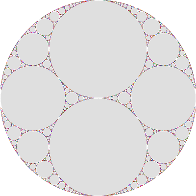
4.82572 x8 - 38.6567 x7 + 124.113 x6 - 203.045 x5 +
178.5 x4 - 83.0921 x3 + 20.855 x2 - 3.88996 x + 1.97609
although I suspect that with more data points, this too might be a fractal curve.
The Riley slice
Using the Riley parameter λ and method 3 above,
Any two groups in the Riley slice with the same values of the invariant
tr(ab) - 2
up to sign, are conjugate (Lyndon and Ullman).
This implies that the slice is symmetrical about both the real and imaginary axes.
In the montage below, I have sampled the region between the origin and 2+i in increments of 0.1 and 0.1i;
as above, each sample is centered on its coordinate (zmax drops from 21.05 near the origin to √2,
approximately as one over the square root of the distance from the origin):
(Nmin = 424, Nmax = 482,529; color contours range from red = Log10Nmin to violet = Log10Nmax)
The origin is the modular group; the remaining limit sets on the real axis seem to be conjugate to the modular group, at least for rational λ. Most of the region near the origin contain non-discrete groups, with the exception of what appears to be a non-free group at λ=i/2:
(zmax = 3.864)
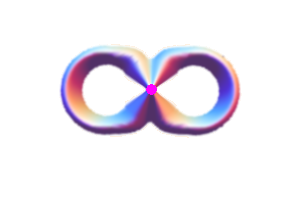
The group at λ=i is a conjugate of the Apollonian gasket; this is the only group relation between the Maskit and Riley slices:
(zmax = √2)
In the point density plot below, I have explicitly shown the axial symmetries of the Riley slice. The plot covers the region -2 ≤ Re(λ) ≤ 2 and -1 ≤ Im(λ) ≤ 1. The dotted line outlines the boundary of the region containing non-discrete groups. It is not known that the boundary is fractal, but more detailed plots (Gilman) would suggest that this is true. As we have seen above, there appear to be non-discrete groups outside the plotted region.
Lyndon and Ullman showed that groups of the Riley slice are free for all groups outside the solid lines. The isolated black points near the blue/magenta boundary locate the figure 8 knot complement. The white points appear to be non-free groups:
(zmax = 3.836)
The slice where both a and ab are parabolic
Using method 5 above, tr(b) is the free parameter, tr(a) and tr(ab) are of course 2, and using
tr(abAB) = tr(a)2 + tr(b)2 + tr(ab)2 - tr(a) tr(b) tr(ab) - 2(Mumford et. al.), we have
 ........
 ........
 ........
 ........
 ........

 ........
 ........
 ........
 ........
 ........
 ........
 ........
 ........