
Continuous spectra is that rainbow of colors displayed by sunlight passing through a prism. It results from the black body thermal radiation generated deep within the Sun:
The location of the peak and overall shape of the curve are determined by the the surface temperature of the star in Kelvin (= Celsius + 273.15).
Emission spectra are the bright lines generated by electron transitions. Absorption spectra are dark lines in the continuous spectrum caused when an atom or molecule absorbs a photon, and one of its electrons jumps to a higher energy level. Absorption lines are widely used in astrophysics, allowing the investigation of chemistry on other worlds and chemical makeup and nuclear processes in stars from our own Sun to those literally across the universe.
The spectral data varies in resolution and coverage among the stars: some spectra include ultraviolet and/or infrared wavelengths while others cover only part of the optical spectrum. All are flux-calibrated spectra, meaning that the flux values have calibrated physical units of Watts per square meter per Angstrom. Some of the original spectra were compiled at resolutions greater than the applet's finest resolution of one value per Angstrom, and those spectra have been smoothed for our use here. In addition, some spectra have been truncated because of the applet's limited color resolution: it can show only 256 levels of intensity for any given hue.
Begin by choosing a star from the pop-up menu. An image of the star will be displayed and, for most stars, the measured annual parallax angle and absolute error in that measurement will be displayed in the text box to the right of the image.
Note that the image is not, except in the case of Sol, an image of the stellar surface. It is actually a diffraction pattern (interference pattern) with a strong, wide central maximum (the central circular "image") and in most cases indiscernible secondary maxima. In most cases, diffraction spikes will be visible; these indicate that the star is relatively close to us.For all stars, the text box will also contain the minimum and maximum flux values over the range of the displayed spectrum, along with the total flux over that range.
Below this is another pop-up menu which selects an element (or ion or molecule) for spectral line identification, followed by a button and scroll bar enabling a black body temperature fit to the spectrum. Beneath those are three displays. The top display shows the spectral lines associated with the element selected (they are displayed as emission lines, that is, bright against a black background). Below that is a reconstructed color image of the actual spectra (wavelengths in the ultraviolet and infrared are displayed in shades of gray). Finally there is a graph of the flux as a function of wavelength:
You may click on either the spectrum image or graph to mark a central wavelength value on which to focus for detailed inquiries. The "Zoom In" and "Zoom Out" buttons allow you to quickly change the range of wavelengths displayed about that central value, and the values of the wavelength at the left and right edges of the graphs are displayed to the right of those buttons. The scroll bar labeled "Central lambda" allows you to smoothly vary the central value, and the value of the flux at the central wavelength is displayed to the right of the central lambda value. Finally, the "Gaussian Fit" button draws a Gaussian fit to the spectrum graph centered on the central lambda value, with a standard deviation (half-width) as specified by the scroll bar to the right.
(source, source, source, source, source, source, source)
energy flux = luminosity / (4 π distance2)Using values from the Spectrum Viewer for the star 108 Virginis, we see from its parallax (5.31 mas) that its distance from Earth is
r = 1000 pc/mas / 5.31 mas = 188.3 pc, times 3.086 * 1016 m/pcThe Viewer also tells us that its total flux is 9.9775 * 10-11 W/m2, so its luminosity is= 5.81 * 1018 m
L = 4 π * (5.81 * 1018 m)2 * 9.9775 * 10-11 W/m2Note that we do not have a "complete" spectrum; there appears to be additional flux in the ultraviolet that is missing from the data for this star. Because of this, we have really underestimated the luminosity of this star.= 4.23 * 1028 W, divided by 3.84 * 1026 W for our Sun= 110 Lsolar
We can find the effective temperature of a star as follows. Use the "Black Body" button and adjust the temperature scroll bar so that the black body curve is as close to the spectrum as possible. Since a star is not a perfect black body, we have some choices here: we can match the peak wavelength (in this example, around 3970 Angstroms, giving us a temperature of 7300 K) or we can match the leading or trailing slope (in this example, closer to 9300 K). In general, matching the trailing slope tends to be more accurate than the other options.
A given atom, ion or molecule only exists in a star's atmosphere for a range of temperatures. At lower temperatures, an ion may capture one or more free electrons to become neutral. At higher temperatures, collisions may cause an atom to lose one or more electrons to become ionized. In either case, this will change the wavelengths of its absorption lines. At sufficiently high temperatures, molecules will break up into their constituent atoms, and their lines (or bands) disappear altogether. We can use the following table to look for some characteristic lines as a check on our black body temperature. Choose the element from the drop-down menu ("Reference Spectra Element") and look for consistent matches for the lines displayed, indicating the presence of that element in the star's atmosphere. If the lines in the table are present, the temperature should be in or close to the range given, and if the lines are extremely strong (dark), the temperature should be close to the peak temperature. The wavelengths for the CH and TiO bands are the wavelengths at the left-hand edge of the bands.
| specie | lines (Angstroms) | T Range (K) | Peak T (K) |
|---|---|---|---|
| H | 3966, 4097, 4336, 4856, 6555 | 5000-40000 | 9000 |
| He | 4471, 4542 | 10000-50000 | 29000 |
| Ca | 4227 | 2000-5500 | 3000 |
| Ca+ | 3934, 3968 | 3000-7000 | 5000 |
| Na | 5890, 5896 | 2000-5500 | 3000 |
| Mg+ | 2796, 2802, 4481, 5173 | 8000-30000 | 9200 |
| Si+ | 4128, 4131 | 8000-20000 | 9200 |
| Si++ | 4552 | 20000-40000 | 25000 |
| Si+++ | 1394, 1403, 4089, 4116 | 30000-50000 | 40000 |
| Fe | 4045, 4143, 4299, 4325, 4384, 5270 | 2000-7000 | 4500 |
| Fe+ | 4173, 5316 | 4000-8000 | 5700 |
| CH band | 4300-4315 | 5000-6000 | 5500 |
| TiO bands | 4762, 4955, 5167, 5448, 5862, 6159, 6384 | 2000-4000 | 3000 |
Here are sample optical spectra arranged by spectral class; can you identify the prominent lines?
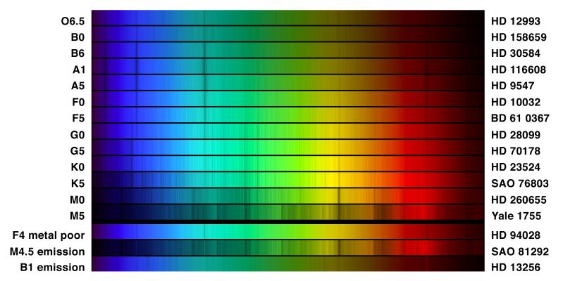
The spectrum for 108 Virginis is a low resolution spectrum, so all we can see are the broad Hydrogen lines, which do not help much in verifying our black body temperature. This check is much more useful with high resolution spectra, especially spectra in the visible and near ultraviolet.
With the temperature and the luminosity, we can compute the star's radius using
luminosity = 4 π σ radius2 temperature4Using our temperature of 9300 K for 108 Virginis (and 5.67 * 10-8 for σ), we obtain
r = (4.23 * 1028 / 4 π σ 93004)1/2Since our estimate for the luminosity was low, this is an underestimate for the radius. But because of the square root, we are closer here than in our luminosity calculation (if the luminosity was off by a factor of 2, the radius will only be off by a factor of 21/2 = 1.414).= 2.82 * 109 m, divided by the radius of our Sun (7 * 108 m)= 4 rsolar
Note that the presence of metallic absorption lines indicates that the star is a later-generation star: the metals were inherited from earlier-generation stars.
For one or more of your stars, the applet may not have parallax information; for these you will only be able to find the black body temperature.
Several of the spectra show strong emission lines (associated with flares) which alter the scale of the graph and make
black body temperature estimation more difficult.
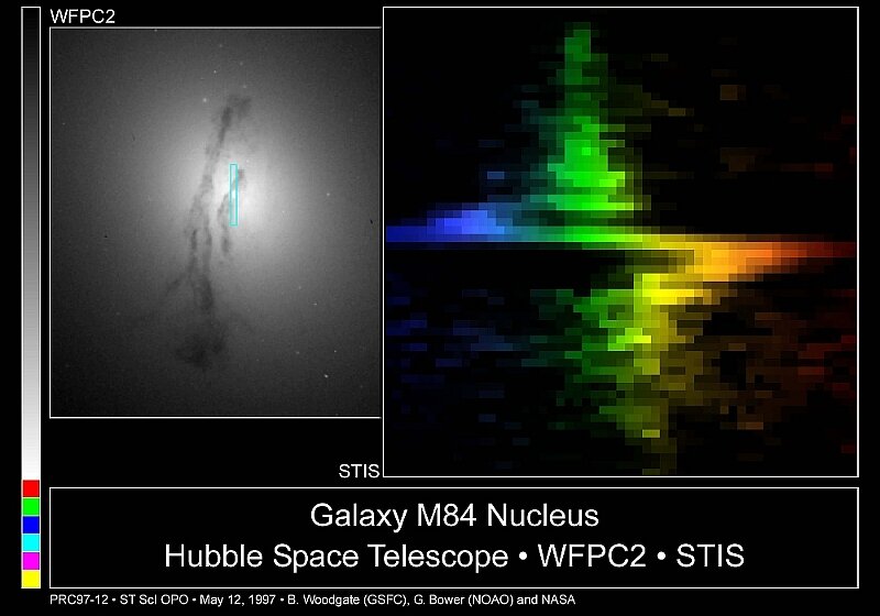
A dramatic illustration of the Doppler effect provided some of the first real evidence for the existence of black holes.
Since recessional motion (away from us) causes the apparent wavelength to be larger, color is shifted toward the red end of the spectrum;
this is called red shift. If the source is moving toward us, the apparent wavelength will be smaller, and color
will be shifted toward the blue end of the spectrum: blue shift. When red and blue shifted light comes from
adjacent areas in a very small region of the center of a galaxy, it is a signal that matter is rotating very quickly around a compact
object. In this case, the only type of object expected to be able to cause rotational motion of that magnitude is a black hole.
The Spectrum Viewer does not have sufficient resolution to enable us to compute recession shifts for any of the stars
it has data for. But we will return to this computation when we discuss Cosmology.
The broadening of most narrow absorption lines is primarily due to the motion of the atoms involved, although pressure and
other factors can be equally important. For instance, Hydrogen and Helium lines are broadened by the Stark Effect:
since their nuclear charge is small,
they are particularly susceptible to electric fields created by ions in the stellar atmosphere. These fields perturb their energy levels and
are primarily responsible for their line broadening.
Atomic speeds in the photosphere can be estimated using the width of some absorption lines:
The spectrum for 108 Virginis has too low a resolution to be able to compute Doppler Shifts; only the broad Hydrogen lines are present,
and these are unsatisfactory for computing atomic velocities, because of the Stark Effect. But using the prominent Sodium line of
Epsilon Indi (at 5890 Angstroms), we can compute an approximate speed for these atoms in the star's atmosphere as follows. Click on the
graph at 5890 Angstroms, and "Zoom In"; if the central wavelength is not 5890, click again or use the "Central Lambda" scroll bar until it is.
Then click the "Gaussian Fit" button; a small curve appears around the line. Change the Standard Deviation using the scroll bar until the
curve is a close fit to the line on the graph. In this example, it is a close fit between 1.5 and 2.4.
Taking the average (1.95), we compute the approximate speed of these atoms as
energy flux, luminosity, distance, absolute magnitude (M) and apparent magnitude (m). So in principle, if we know any two of these
quantities, we can use the three equations to compute the others. Photometry gives us the energy flux and apparent magnitude, so
we seem to be home free. But there is an assumption that we have ignored, and which we must take into account: space is not
entirely empty.
The volume in the immediate neighborhood of the Earth has a mean density of about 5 atoms per cubic centimeter (mostly
Hydrogen (source); 1 cm3 = 10-6 m3).
This falls to about 0.3 in the
Solar neighborhood and to less than 0.001 in the "Local Bubble":
In interstellar space the average density is around
1 atom per cm3, and it is even less in intergalactic space. Larger dust particles are about a million times rarer,
except in nebulae and clouds, where the density runs between 10 to a million atoms, molecules or dust particles per cm3.
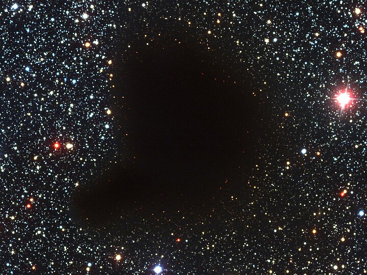
But since space is so vast, some of the electromagnetic
radiation traveling through the interstellar medium is absorbed, and because shorter wavelengths are scattered more than
longer ones, there is additional attenuation in the red and infrared wavelengths. The overall loss is called extinction, and
the preferential scattering causes reddening. The following
absorption nebula illustrates both phenomena:
While the spectra in the Spectrum Viewer have been corrected for extinction and reddening, it is important to know how
astronomers can compute the necessary corrections. Armed with an independent measure of distance (for instance, from the parallax),
we can compare the observed apparent magnitude with the expected apparent magnitude. The result is
Spectral classification is particularly useful here. Along the main sequence of a Hertzsprung-Russell diagram, there is
essentially a 1:1 correspondence between spectral class and absolute magnitude. Because of this, stars of a given spectral class
but at various distances can be used to compute extinction. For instance, the star BD +31 640 is located in the open
galactic cluster IC 348. It is an A3V star located 236 parsecs away, with an absolute magnitude of 1.5. This means the expected
apparent magnitude (m = M - 5 + 5 log D) is
Portfolio Exercise:
You will be given a list of 9 stars which you are to analyze for several portfolio exercises. In this exercise,
Doppler Shift
Line of sight motion can be computed using the shift in the central wavelength of well-known absorption lines:
apparent wavelength / actual wavelength = 1 + recession velocity / c
If the apparent wavelength is shorter than the actual, the motion is toward us and the recession velocity is taken to be negative.
Red and blue shift in the nucleus of M 84 signals the presence of a black hole. (source)
line width = 2 * speed * central wavelength / c
The line width is twice the standard deviation reported by the Spectrum Viewer.
v = 1.95 * 3 * 108 / 5890 = 99000 m/s
Portfolio Exercise:
Using both the Calcium lines near 3900 Angstroms, and the Sodium lines near 5900 Angstroms, compute the approximate atomic speeds from the
line width, for each star.
If the lines are not clearly defined and relatively deep, it will not be possible to do this. This will occur
if one or more of your stars have low-resolution spectra, or those lines are located in very low-flux wavelengths. List those
stars which you are unable to evaluate.
Are the speeds consistent for each star? What does the range tell you about this computation?
Extinction
Taking inventory of our equations involving luminosity and magnitude, we see that we have three equations in five unknowns:
Our Sun's neighborhood in the Milky Way. (source)
 Molecular Cloud Barnard 68, showing both extinction and reddening. (source)
extinction = (mobserved - mexpected) / distance
here measured in magnitudes per kiloparsec; note that it is a function of wavelength.
1.5 - 5 + 5 log 236 = 8.36
However, the observed apparent magnitude (measured near 5448 Angstroms, the effective wavelength for the V band) is 11.4
(source), meaning that the extinction
is
(11.4 - 8.36) / 0.236 = 12.86 magnitudes / kpcIn this case, the extinction is due largely to an obvious cloud:
and it is more reasonable to quote the extinction simply as 3.04 magnitudes.
©2010, Kenneth R. Koehler. All Rights Reserved. This document may be freely reproduced provided that this copyright notice is included.
Please send comments or suggestions to the author.