
| (prev) | (top) | (next) |
Electric charge is the source of the electric field.
A field is a smooth function which has a value at every point in space.
The value may be a scalar or a vector.
Assuming a uniform medium, ε is the electrical permittivity, often written as
V is measured in Volts; 1 V = 1 J / C, so the electrical potential energy of a charge at a point in space is
This applet will allow you to experiment with the potentials due to various charge configurations.
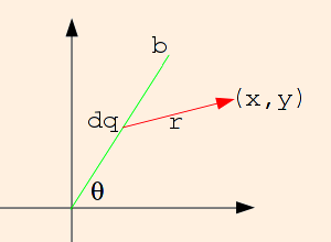
Consider a wire of length b, with constant linear charge density λ, extending from the origin at an angle θ:
Choosing the field point
to be (x, y), and calling the distance from the origin to the source point (along the wire) "s", we have
r = √ (s2 + x2 + y2 - 2 s (x cos θ + y sin θ))
= (λ / (4 π ε)) ln ((b - a + √ (b2 + x2 + y2 - 2 b a)) /
(√ (x2 + y2) - a))
= (λ / (4 π ε)) (ln ((b - x + √ ((b - x)2 + y2)) / (√ (x2 + y2) - x)) +
Electrical Potential
V(x,y,z) = (1 / (4 π ε)) ∫ dq / r
where the integral is a sum over all of the charges and the denominator of the integrand is the distance from each bit of charge to the
field point (x,y,z).
ε ≡ κ ε0,
where κ is the dielectric constant (≥ 1) and ε0 is the permittivity of the vacuum,
equal to 8.8542 * 10-12 C2 / (N m2). The permittivity is a measure of how "effective" the field is in the medium.
U = qt V
where qt is the test charge: an artifice used to measure the field without contributing to it.
Think of the electric potential as the potential energy per unit charge at every point in space.
ρ ≡ Q / V,
so that in the integrals for the field:
σ ≡ Q / A, or
λ ≡ Q / L,
dq = ρ dV,
Note that dl, dA and dV are implicitly positive; when expressing them in terms of coordinates, pay close attention to integration limits!
Check yourself by noting that V should have the same sign as the charge density involved.
dq = σ dA, or
dq = λ dL.
r = (x - s cos θ, y - s sin θ)
Since s is manifestly positive, dq is equal to λ ds. So
V(x, y) = (1 / (4 π ε)) ∫0b λ ds / √ (s2 + x2 + y2 - 2 s (x cos θ + y sin θ)).
Substituting
u = s - (x cos θ + y sin θ)
will put this integral into a simpler form (since the quantity in parentheses is
a constant with respect to the integration variable, we have chosen to call it "a"). Since ds = du, integrating gives us
= s - a
V(x, y) = (1 / (4 π ε)) ∫- ab - a λ du /
√ (u2 + x2 + y2 - a2)
We can easily compute the potential due to a line of charge extending from (-b,0) to (b,0) as
= (λ / (4 π ε)) ln (u + √ (u2 + x2 + y2 - a2)
|- ab - a
(Note that this derivation fails if the field point is collinear with the wire; but of course, that is an easy special case to do "by hand"!)
V(x,y) | θ=0 + V(x,y) | θ=π
If the field point is on the y axis, this becomes
= V(x,y) | a=x + V(x,y) | a=-x
ln ((b + x + √ ((b + x)2 + y2)) / (√ (x2 + y2) + x)))
= (λ / (4 π ε)) ln ((b - x + √ ((b - x)2 + y2))(b + x + √ ((b + x)2 + y2)) / y2).
(λ / (2 π ε)) ln ((b + √ (b2 + y2)) / y).
| (prev) | (top) | (next) |
©2011, Kenneth R. Koehler. All Rights Reserved. This document may be freely reproduced provided that this copyright notice is included.
Please send comments or suggestions to the author.