color[y_] := Block[ {x, v, i}, (The color function assigns colors to specific ranges of values taken by the scalar field. It assumes that the variables smin and smax have been initialized with the minimum and maximum values to be plotted; both it and the dplot function which calls it use a logarithmic scale. For positive values, blue < green < red < white, which corresponds to smax. For negative values, cyan > yellow > magenta > white, which corresponds to -smax. Black corresponds to zero.x = Log [10, Abs[y]];dplot[ x_, mm_, rr_, zz_] := Block[ {pp, r, c}, (If[ x > smax, i = 4,
If[ x > (smin + 2sd / 3), (i = 3; v = Abs[ 3(x - (smin + 2sd / 3)) / sd];),If[ y >= 0, Switch[i,If[ x > (smin + sd / 3), (i = 2; v = Abs[ 3(x - (smin + sd / 3)) / sd];),
If[ x >= smin, (i = 1; v = Abs[ 3(x - smin) / sd];),]]]];
Return[z];)];1, z = RGBColor[0, 0, v],Switch[ i,2, z = RGBColor[0, v, 0],
3, z = RGBColor[v, 0, 0],
4, z = RGBColor[1, 1, 1]],
1, z = RGBColor[0, v, v],2, z = RGBColor[v, v, 0],
3, z = RGBColor[v, 0, v],
4, z = RGBColor[1, 1, 1]]];
pp = 100;r := Sqrt[rho^2 + zed^2];
c := zed / r;
tab = Flatten[ Table[ Table[ Abs[x], {rho, rr / pp, rr, rr / pp}], {zed, zz / pp, zz, zz / pp}]];
smin = If[ Min[tab] > 0, Log[10, Min[tab]], 0];
smax = mm * Log[10, Max[tab]];
sd = smax - smin;
Print[ "Range = (", Min[tab], ",", Max[tab], "), scale is Log\n",
"blue < green < red < white (values < 0, cyan > yellow > magenta > white)"];gtab = Flatten[ Table[ Table[ {color[x],Rectangle[ {rho - rr / (2pp), zed - zz / (2pp)}, {rho + rr / (2pp), zed + zz / (2pp)}]},Show[ Graphics[gtab], Axes -> True, AxesOrigin -> {0, 0}];)];{rho, rr / pp, rr, rr / pp}], {zed, zz / pp, zz, zz / pp}]];
The dplot function plots values in the first quadrant of the ρ-z plane. It accepts four arguments: the scalar field to be plotted, a scale factor which can be used to produce the greatest color variation in regions of interest, and the maximum limits of both ρ and z. It creates the image by drawing a series of rectangles, each of whose color is determined by the scalar field value in the center of the rectangle. The variable pp can be modified to produce more or less resolution.
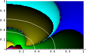
For example, we plot here the Kretschmann Invariant and Ra b c d; e Ra b c d; e for a near-extreme Kerr-Newman metric. The white lines indicate the positions of the horizons:
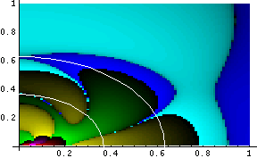
The maximum values for these plots are 1.19 * 108 and 6.83 * 1012, respectively. For comparison purposes, we plot the Kretschmann invariant and Ra b c d; e Ra b c d; e for a near-extreme Kerr metric:
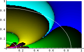
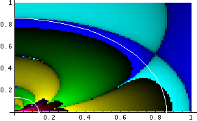
The maximum values for these plots are 2.65 * 107 and 5.9 * 1011, respectively. Note the cyan-blue border which extends from about (0, 0.8) to about (1, 0) in the plot on the right: this is the ergosphere, and the border shows the change in sign which Ra b c d; e Ra b c d; e undergoes as one crosses it.
Here is the Mathematica code to generate the first plot above; note that all parameters other than those defined by the coordinates r and c must be specified before plotting can be done:
params = {A -> Sqrt[2] / 4.1, M -> .5, e -> Sqrt[2] / 4.2};pp1 and pp2 give the horizon lines. The second two plots correspond topp1 = ParametricPlot[
{(M + Sqrt[M^2 - A^2 - e^2] /. params) Sqrt[1 - c^2],pp2 = ParametricPlot[(M + Sqrt[M^2 - A^2 - e^2] /. params) c}, {c, 0, 1},
AxesOrigin -> {0, 0}, PlotStyle -> RGBColor[1, 1, 1]];
{(M - Sqrt[M^2 - A^2 - e^2] /. params) Sqrt[1 - c^2],dplot[kr /. params, 1, 1, 1];(M - Sqrt[M^2 - A^2 - e^2] /. params) c}, {c, 0, 1},
AxesOrigin -> {0, 0}, PlotStyle -> RGBColor[1, 1, 1]];
Show[ {Graphics[gtab], pp1, pp2}, Axes -> True, AxesOrigin -> {0, 0}];
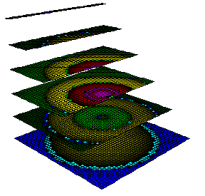
params = {A -> Sqrt[2] / 4.1, M -> .5, e -> 0};It is sometimes useful to visualize a scalar field in three dimensions, but two techniques are necessary in order to do this effectively: the plot must be generated as a series of parallel planes, and the planes must be cut away so that the detail of lower planes can be seen. The following Mathematica code can be used to generate a three dimensional plot:
dplot3D[ expr_, mm_, ll_, ss_, xx_, yy_, zz_] := Block[ {pp, r, c, tab, xc, yc, zc}, (Note that dplot3D is essentially the same as dplot. It accepts seven arguments: the scalar field to be plotted, the color scale factor, the number of layers, the slope of the cutaway plane (implemented in the iterator for the y coordinate), and the maximum x, y and z values to be plotted. For example:pp = 40;r := Sqrt[(xc + xx / pp)^2 + (yc + yy / pp)^2 + zc^2];
c := zc / r;
tab = Flatten[ Table[ Table[ Table[ Abs[expr],
{xc, -xx, xx, 2 xx / pp}],smin = If[ Min[tab] > 0, Log[10, Min[tab]], 0];{yc, -yy + 2 (pp - 1) yy (zc + zz) / (2 zz * pp * ss), yy, 2 yy / pp}],
{zc, -zz, zz, 2 zz / ll}]];
smax = mm * Log[10, Max[tab]];
sd = smax - smin;
Print[ "Range = (", Min[tab], ",", Max[tab], "), scale is Log\n",
"blue < green < red < white (values < 0, cyan > yellow > magenta > white)"];gslice = Graphics3D[ Flatten[ Table[ Table[ Table[Lighting -> False, Boxed -> False];{color[expr],{xc, -xx, xx, 2 xx / pp}],Polygon[ {{xc, yc, zc}, {xc + 2 xx / pp, yc, zc},
{xc + 2 xx / pp, yc + 2 yy / pp, zc}, {xc, yc + 2 yy / pp, zc}}],
Thickness[.001]},
{yc, -yy + 2 (pp - 1) yy (zc + zz) / (2 zz * pp * ss), yy, 2 yy / pp}],
{zc, -zz, zz, 2 zz / ll}]],
Show[ gslice, ViewPoint -> {-2, -2, 1}];)];
dplot3D[ cdrsq /. params, 1, 5, 1, 1, 1, 1];produces the following plot of Ra b c d; e Ra b c d; e for a near-extreme Kerr-Newman metric:
(r < rminus[c * t ,0]) || (r < rplus[c * t, 0]),
PlotRange -> {{0, rend}, {0, tend}},
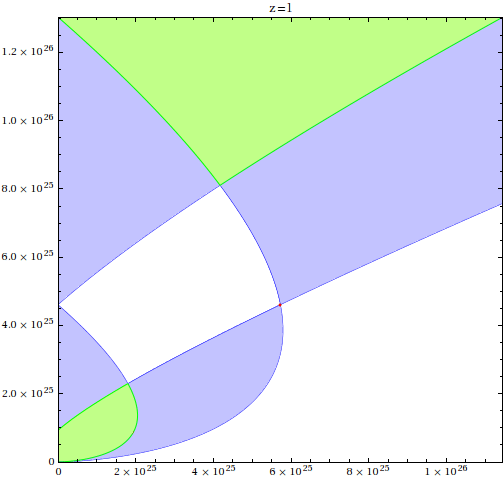
AxesOrigin -> {0, 0}, PlotLabel -> "z=1",
Epilog -> {Red, Point[ {rz1, c * tz1}], Black}],
PlotRange -> {{0, rend}, {0, tend}},
AxesOrigin -> {0, 0}, Frame → False]
The next appendix discusses techniques for functional analysis in Mathematica.
©2014, Kenneth R. Koehler. All Rights Reserved. This document may be freely reproduced provided that this copyright notice is included.
Please send comments or suggestions to the author.
Other Visualizations
Another interesting visualization involves light cones in an expanding universe. Suppose we want to examine light cones for
a pair of events occuring at z=1: one at the origin, and one at rz=1. For a matter-dominated universe, the scale factor is
a(t) = (t / tnow)2/3.
The expansion velocity is
dr(t)/dt = a'(t)/a(t) * r(t)
and so the limits of the light cone are the curves at
dr(t)/dt = a'past(t)/apast(t) * r(t) ± c.
For our a(t), this has the solution
r±(t) = b * t2/3 ± 3 c t.
The constant of integration b is determined for the event at the origin from
r±(tz=1) = 0,
while for the event at rz=1, it is determined by
r±(tz=1) = rz=1.
We can determine tz=1 by inverting the equation for a(t) to get
tz=1 = tnow * a2/3,
with a = 1 / (z + 1) = ½. Suppose that we have previously computed these quantities in Mathematica as
rz1, tz1, rplus[t,0], rminus[t,0], rplus[t,rz1], rmins[t,rz1],
and the plot limits as
rend and tend.
If the speed of light is c, the following code will plot the light cones (with a point at the z=1 event):
Show [RegionPlot [((r > rminus[c * t, rz1]) && (r < rplus[c * t, rz1])) ||
It produces the following plot (timelike light cone interiors are blue, except where they overlap, which is shown in green):
((r < rminus[c * t, rz1]) && (r > rplus[c * t, rz1])) ||
{r, 0, rend}, {t, 0, tend}, PlotPoints -> 200, BoundaryStyle -> Blue,
PlotStyle -> RGBColor[195/255, 195/255, 255/255],
RegionPlot [((r > rminus[c * t, rz1]) && (r < rplus[c * t, 0])) ||
((r > rplus[c * t, rz1]) && (r < rminus[c * t, 0])),
{r, 0, rend}, {t, 0, tend}, PlotPoints -> 200, BoundaryStyle -> Green,
PlotStyle -> RGBColor[193/255, 255/255, 136/255],