
Recall that conservative forces can be written as gradients of potential energy. Just as rates of change over time result in an additional unit of time in the denominator, a gradient results in an additional unit of distance: it is after all a "rate" of change over distance. Since the electric force is conservative, and the electric potential energy has the form
U = q1 q2 / 4 π ε r,we expect the magnitude of the force between two electrically charged objects to be
F = q1 q2 / 4 π ε r2.This force is called the Coulomb force. The direction along which the force acts is on a line directly connecting the two charges. And of course we know that the force can be either attractive, when the charges have opposite sign, or repulsive, when the charges have like sign.
Note that the electrical force between two charges is the same regardless of which we call q1 and which is called q2. We say that the equation for force is symmetric under exchange of the labels.
Just as we used the electric potential to describe the field of a single source charge, we can imagine a force per unit charge due to a source, which we call the electric field:
E (r) = q / 4 π ε r2.
The direction of the electric field is from the location of a positive source charge to the location of the field point (or from the field point to a negative source charge):
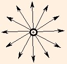
Again, this is due to the spherical symmetry: the only preferred directions are radially inward or outward, and we associate those directions with the sign of the source. The force felt by a test particle in this field is
F = qt Es.This force is of course equal to the Coulomb force; from this equation we can see that the units of the electric field are N / C. The notion here is that a charged particle has an influence independent of whatever forces are felt by other charges.
The electric fields due to multiple sources superpose, as do the forces they exert on a test charge. But because the electric field has direction, the computation of the superposed field must be done using vector components:
Ex = q1 (x - x1) / 4 π ε r13 + q2 (x - x2) / 4 π ε r23and the magnitude of the electric field is thenEy = q1 (y - y1) / 4 π ε r13 + q2 (y - y2) / 4 π ε r23
E = √(Ex2 + Ey2).Here the point (x, y) is the field point, (x1, y1) is the location of q1 and (x2, y2) is the location of q2. The additional factors of (x - xi) / ri and (y - yi) / ri give the cosine and sine of the angle of the line connecting the source charge and the test point; the overall dependence is still 1 / r2. When there is more than one source charge, the direction of the electric field is the same as the direction of the acceleration of a positive test charge at the field point.
Just as the Coulomb force is the gradient of the electrical potential energy, the electric field is the gradient of the electrical potential. Now it is clear why test charges accelerate perpendicularly to equipotentials: the directions of the electric field and force are the same:
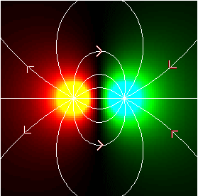
This plot illustrates the electrical potential and field lines of a dipole: a pair of charges with equal magnitude but opposite sign. Here, the positive charge is on the left, and the field lines exit it and enter the negative charge on the right.
The force of gravity is completely analogous to the Coulomb force:
We can now see how to compute the value of g, the "constant" acceleration due to gravity. Approximating the earth by a sphere, we set m2 equal to the earth's mass (mE = 5.974 * 1024 kg) and r to its average radius (rE = 6.378 * 106 m). We can do this because the gravitational field due to a sphere is equivalent to the field of a point source with the same mass at the center of the sphere. The acceleration g of the mass m1 is then the same as the value of the gravitational field at the surface of the Earth:
We now revisit the applet from the last section. We can now find the direction of the electric field, and the magnitudes of the electric field and force, as well as the magnitude of the acceleration. Use the mass of an electron to compute the mass of a negative test charge, and the mass of a proton to compute the mass of a positive test charge.
You should have noticed something interesting while doing the gravitational problems. It should not have been unexpected if you were on your toes:
there is an obvious relation between the units of the gravitational field and those of acceleration, and if you follow the equations you used
to analyze the problems, the reason should be clear. This relation has deep roots: Einstein's
General Theory of Relativity tells us in part that gravity is indistinguishable from acceleration.
In the next section, we begin our application of these concepts to electrical circuits.
©2013, Kenneth R. Koehler. All Rights Reserved. This document may be freely reproduced provided that this copyright notice is included.
Please send comments or suggestions to the author.
Gravitational Forces
F = - G m1 m2 / r2.
Note that gravitational forces are always attractive, since mass is always positive. In exactly the same way
as with the electric field, we can define a gravitational field whose units are N / kg.
G mE / rE2,
or approximately 9.8 m / s2!