initcond[ t_, x0_List, xdot0_List] := N[ Table[ {x[[i]][t] == x0[[i]],The geointegrate function has as arguments the list of initial conditions (as supplied by initcond), the starting and ending "times", which are actually affine parameter values, and the number of integration steps. The latter, as well as the precision specifications, must often be adjusted for sufficient accuracy near rapidly oscillating or singular regions. The initcond and geointegrate functions cooperate in referring to the positions using the variable "x", but the NDSolve function will return a function of the affine parameter "ap". We turn off the precw error in order to create slightly cleaner output. Note the use of the N function to force numerical evaluation: numerical integration requires that ALL symbols have numerical values.x[[i]]'[t] == (xdot0[[i]] /. Thread[ x -> x0])}, {i, 4}]];geointegrate[ initialconds_List, tstart_, tend_, steps_] := Block[ {x},(x = xk;geodesiceqs = Table[ N[ D[ D[ x[[ii]][ap], ap], ap] + Simplify[ Sum[ Sum[
(christoffel[[ii, jj, kk]] /. Thread[ x -> Table[ x[[ll]][ap], {ll, 4}]]) *{kk,4}], {jj, 4}]]] == 0, {ii, 4}];D[ x[[jj]][ap], ap] * D[ x[[kk]][ap], ap],
Off[ NDSolve::precw];
soln= NDSolve[ Flatten[ {geodesiceqs, initialconds}], x, {ap, tstart, tend},
MaxSteps -> steps, WorkingPrecision -> 2 $MachinePrecision,Return[soln];)];PrecisionGoal -> $MachinePrecision];
It remains to do the actual integration, setting the mass of the Schwarzschild source at 5 Solar Masses
and converting that mass to the geometrical units used in the metric:
G = 6.673 * 10^(-11);
mass[m_] := m * G / c^2;
Msolar = 2 * 10^30;
M = mass[ 5 Msolar];
headpath = geointegrate[ initcond[ 0, head, headdot], 0, 1, 1000];
8.52599928623598130422369177215748897726102`31.909179540382006*^-6. More...
5.910415200172342049582861192500640452333204`31.909179540382006*^-6. More...
We want to plot both geodesics in such a way that we can compare their positions at any given
affine parameter. We will also want to include the horizon and central singularity in the plot.
The following sequence of Mathematica code (with interspersed commentary) accomplishes this:
The plotgeo function below also takes the
geointegrate output as an argument, as well as the horizontal and vertical coordinate ranges for the
plot, and the affine parameter range for the geodesic:
domain = Evaluate[ Flatten[ {ap, (x[[1]] /. path[[1, 1]])[[1]]}]];
function = Evaluate[ Flatten[ {x[[1]][ap], x[[dim]][ap]} /. path]];
nseg = 120;
dap = (domain[[3]] - domain[[2]]) / nseg;
api = domain[[2]];
Do[( AppendTo[ps,
Graphics[
PlotRange -> {xlim, ylim}, PlotPoints -> 2,
DisplayFunction -> Identity]];
AppendTo[ ps,
PlotStyle -> {RGBColor[0,0,1], RGBColor[0,0,0], Dashing[{0.05, 0.05}], Dashing[{0.05, 0.05}]},
DisplayFunction -> Identity]];
Return[ps];)];
DisplayFunction -> $DisplayFunction], ImageSize -> 400,
AxesOrigin -> {If[ xlim[[1]] < 0, 0, xlim[[1]]],
If[ ylim[[1]] < 0, 0, ylim[[1]]]};
Tlim = {0, 1.1};
headgeo = plotgeo[ headpath, Xlim, Tlim, {0, endpoint[ feetpath]}];
feetgeo = plotgeo[ feetpath, Xlim, Tlim, {0, endpoint[ feetpath]}];
kruskalgeo = plotkruskal[ Xlim, Tlim];
showgeo[ {feetgeo, headgeo, kruskalgeo}, Xlim, Tlim];
The geodesic on the left is the path of the foot of the rod, while the one on the right is that of the head.
The color of both geodesics starts at red, and the fact that the head geodesic ends at magenta instead of
blue indicates that a longer affine parameter "time" has elapsed when the head reaches the central
singularity as compared to the foot: of course, the foot hits first. The affine parameter of the foot
as it crosses the upper dashed line is the same as that of the head as it crosses the lower dashed line.
We see that the rod is stretched by computing the distance between the two lines:
from its original 100, it has grown to over 3400 meters!
It is a good exercise to examine the Kerr geodesics numerically.
Because the symmetry is axial, the initial orientation of the rod allows for interesting variations, and you
will want to examine the geodesics in all of the spacelike planes (in plotgeo,
the variable "function" determines
the coordinate variables used in the plot). It is interesting to note that the
angular momentum parameter must be very nearly equal to the mass parameter before most of the rotational
effects become obviously visible in the graphs. Note that you may have to increase the number of steps due to
ndsz errors, in which the step size becomes effectively zero.
Sometimes it is useful to take matters into your own hands in order to avoid issues with singularities, or simply
singular coordinates. The following example shows how to solve the geodesic equation for r'(φ) (previously defined as rpphi[r]) using the
Runge-Kutta method, and plot the resulting geodesics:
geoplotRK[ r0_] := Block[ {}, (
dphi = Pi / 100;
ri = r0;
phii = phi0;
While[ ( ri < 2 rmax ) && ( phii < 3 Pi / 2 ), (
k2 = dphi * rpphi[ ri + k1 / 2];
k3 = dphi * rpphi[ ri + k2 / 2];
k4 = dphi * rpphi[ ri + k3];
r2 = ri + ( k1 + 2 k2 + 2 k3 + k4 ) / 6;
AppendTo[ ps, Graphics[ Line[ {{ ri * Cos[ phii], ri * Sin[ phii]}, { r2 * Cos[ phii + dphi], r2 * Sin[ phii + dphi]}}]]];
ri = r2;
phii = phii + dphi;)];
dphi = - Pi / 100;
ri = r0;
phii = phi0;
While[ ( ri < 2 * rmax ) && ( phii > - Pi / 2 ), (
k2 = - dphi * rpphi[ ri + k1 / 2];
k3 = - dphi * rpphi[ ri + k2 / 2];
k4 = - dphi * rpphi[ ri + k3];
r2 = ri + ( k1 + 2 k2 + 2 k3 + k4 ) / 6;
AppendTo[ ps, Graphics[ Line[ {{ ri * Cos[ phii], ri * Sin[ phii]}, { r2 * Cos[ phii + dphi], r2 * Sin[ phii + dphi]}}]]];
ri = r2;
phii = phii + dphi;)];)];
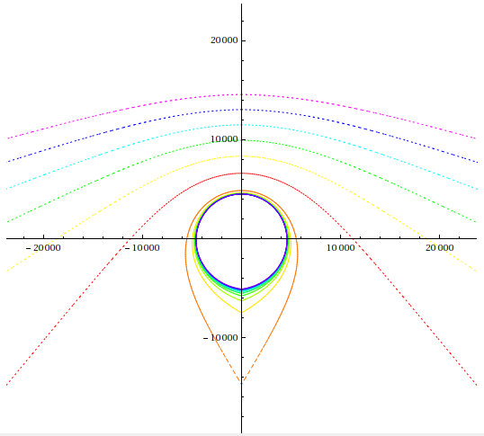
Here we see two families of geodesics: the solid lines represent Λ=0 (b/M taking values from 6 to 11), and the dashed lines represent Λ<0
(LAdS/M taking values from 0.3 to 3, inner to outer, with b/M just larger than the smallest allowable value).
ac = - a2 c (e2 - 2 M r) /
((a2 c2 + r2) (a2 c2 + e2 - 2 M r + r2))
ωr φ = - a (1 - c2)
(a2 c2 M + e2 r - M r2) /
((a2 c2 + r2)1/2
(a2 c2 + e2 - 2 M r + r2)3/2)
ωc φ = a c (- e2 + 2 M r)
(a2 + e2 - 2 M r + r2) /
((a2 c2 + r2)1/2
(a2 c2 + e2 - 2 M r + r2)3/2)
c = 2.98 * 10^8;
The mxst error occurs when the geodesic reaches the central singularity. Choices of starting
and ending times are arbitrary, but their difference must be sufficient to get you where you want to go.
NDSolve::"mxst" : Maximum number of 1000 steps reached at the point ap ==
feetpath = geointegrate[ initcond[ 0, feet, feetdot], 0, 1, 1000];
NDSolve::"mxst" : Maximum number of 1000 steps reached at the point ap ==
endpoint[ path_] := (x[[1]] /. path[[1,1]])[[1,1,2]];
The output of the geointegrate function is input to the endpoint function, which simply finds the
value of the affine parameter at the "end" of the geodesic. This and the functions below also
cooperate with geointegrate in using the "x" variable defined there.
plotgeo[ path_, xlim_List, ylim_List, plim_List] := Block[ {ps, api},(
This function creates a list of Graphics objects. The odd numbered objects in the list set the color
for that segment of the plot, while the following object is the plot of that segment.
In this manner, the color of the geodesic plot relates directly to the value of the affine parameter
there. The variable "nseg"
defines the number of segments in the plot. The "DisplayFunction -> Identity" specification prevents
ParametricPlot from displaying the segments as individual plots.
ps = {};
Return[ps];)];
Hue[ FractionalPart[ (api - domain[[2]] +
plim[[1]]) / (1.5 plim[[2]])]]]];
AppendTo[ ps, ParametricPlot[
Evaluate[ function], {ap, api, api + dap},
api = api + dap;),
{k, nseg}];
plotkruskal[ xlim_List, ylim_List] := Block[ {ps},(
plotkruskal simply creates the plots for the central singularity and the horizon, along with
two dashed lines for distance comparisons, and then changes the
plot color back to black so that the axes and labels will display. showgeo is then used
to display the list of plots overlayed as a single graph:
ps = {};
Plot[ {Sqrt[1 + X^2], X, Sqrt[.7715 + X^2], Sqrt[.4664 + X^2]},
AppendTo[ ps, Graphics[ RGBColor[0, 0, 0]]];
{X, xlim[[1]], xlim[[2]]},
PlotRange -> {xlim, ylim},
showgeo[ ps_, xlim_List, ylim_List] := Show[ ps,
These functions are used as follows:
PlotRange -> {xlim, ylim}, Axes -> True,
Xlim = {.1, .28};
to generate this plot:
ps = {};
Here, we integrate first from π/2 to 3π/2, then from π/2 to -π/2. Each integration starts at the same distance r0 because it is the
common starting point for each half of the trajectory (although it is obviously the mid-point of the geodesic.) This code was used to plot the geodesics
for the Schwarzschild/Anti-deSitter black hole in D=4:
phi0 = Pi / 2;
k1 = dphi * rpphi[ ri];
phi0 = Pi / 2;
k1 = - dphi * rpphi[ ri];
Acceleration, Expansion, Shear and Twist
A unit (or null) vector ua tangent to a geodesic may be analyzed in terms of four quantities:
The covariant derivative of a vector can be
decomposed in terms of these quantities:
ab = uc ub; c,
measuring the component of its derivative parallel to itself;
θ = ub; b,
measuring the tendency of neighboring geodesics to converge or diverge;
σb c = (ab uc +
ac ub + ub; c + uc; b) / 2 -
θ (gb c - |u| ub uc) / (D - n),
(where n = 1 for timelike or spacelike vectors and 2 for null vectors), measuring the tendancy of
neighboring geodesics to accelerate at different rates, and
ωb c = (ab uc -
ac ub + ub; c - uc; b) / 2,
which measures the tendancy of neighboring geodesics to rotate around each other.
ub; c = - ab uc + σb c +
ωb c +
θ (gb c - |u| ub ub) / (D - n)
For instance, for the Kerr-Newman Spacetime,
for the unit asymptotic timelike Killing Vector
ub = {0, 0, 0, - ((r2 + a2 c2) /
(a2 c2 + e 2- 2 M r + r2))1 / 2},
we have (nonzero components)
ar = - (a2 c2 M + e2 r - M r2) /
((a2 c2 + r2) (a2 c2 + e2 - 2 M r + r2))
These are all singular at both the ergosphere and the ring singularity,
as expected since we are dealing with the asymptotic time coordinate. In this coordinate system, all of the
quantities we are computing here are only valid exterior to the outer horizon.
All components save the radial acceleration vanish in the Schwarzschild and
Reissner-Nordstrom limits.
For the inward null radial vector
ub = {-(a2 + e2 - 2 M r + r2)1/2, 0, 0, (a2 c2 + r2) / (a2 c2 + e2 - 2 M r + r2)1/2,all components of both the acceleration and the twist are singular at the ergosphere, and some components of the twist are singular at the horizon. The expansion is singular at both the horizon and the ring singularity, and all components of the shear are singular at one or more of these special locations. No surprises there. In the Schwarzschild limit, we have
ar = r (r - M) / (r - 2 M)In the region of validity for stellar remnant black holes (M > 1/81/2 ~ .0002384 MSolar), the acceleration is positive, the expansion is negative, the shear components in the radial and/or time directions are negative, while those in the angular components are positive, and the r-t twist is positive. These are all consistent with physical expectations: inward radial geodesics (light rays) converge toward the central singularity.at = r - M
θ = - (3 r - 5 M) / (r (r - 2 M))1/2
σr r = - (r - M) (r - 2 M) r1/2 (2 r2 - 1) / (2 (r - 2 M)5/2
σr t = - (2 r3 - 2 M r2 + r - 3 M) / (2 (r (r - 2 M))1/2)
σc c = (r - M) r3/2 / (2 (1 - c2) (r - 2 M)1/2)
σφ φ = (1 - c2) r3/2 (r - M) / (2 (r - 2 M)1/2)
σt t = - (r - 2 M)1/2 (2 r3 - 2 M r2 + 3 r - 7 M) / (2 r3/2)
ωr t = (r - M) / (2 (r2 - 2 M r)1/2)
The next appendix discusses the visual analysis of curvature invariants.
- Table of Contents
- Index:
©2014, Kenneth R. Koehler. All Rights Reserved. This document may be freely reproduced provided that this copyright notice is included.
Please send comments or suggestions to the author.