
Let us start with the simplest of observations: springs bounce. To analyze this phenomenon further, we will simplify the spring in the same spirit as the point particle approximation, and limit its motion to one dimension. Our one dimensional spring can be compressed or extended along the x axis, but cannot be bent or otherwise move in any direction perpendicular to its length.
The first thing that we notice about our spring is that it has a fixed length only when it is not being compressed or extended. This length can be called the spring's equilibrium length, l. It will be convenient to place the spring on the x axis so that one end is anchored at -l, and the other end lies exactly at x = 0 when the spring is at equilibrium.
It is necessary to exert a force on the spring in order to extend or compress it. This force between the spring and the agent acting on it, when measured, is found to be proportional to the displacement x, and in the opposite direction. That is, if the spring (here drawn in red) is compressed a distance x, its free end is at -x and it exerts a force -k x, which is in the positive x direction:
If the spring is extended a distance x, its free end is at x and it exerts a force -k x which is now in the negative x direction:
The constant of proportionality k is called the spring constant, and the relationship
The spring provides us with an opportunity for additional physical analogies. During pulsatile flow, arteries expand and contract with the changes in blood pressure. This movement can be modeled using Hooke's Law, where x is replaced by Δr: the variation in the radius of the artery from its equilibrium position. The aorta typically has a spring constant in the neighborhood of 1000, and radial displacements of around 2 mm.
As usual, we are ignoring friction. As a result Hooke's Law describes a conservative force, which can be written as the gradient of a potential energy. Since the gradient introduces an additional power of distance in the denominator, we expect this elastic potential energy to be proportional to x2. Multiplying by our ubiquitous unitless factor of 1/2, we find that
The spring is a nearly universal model in physics. This is true in part because only it and the 1/r2 force can describe exactly periodic phenomena. As a result, we have the mathematical tools necessary to completely analyze such systems. But the primary utility of the spring goes back to our original observation: it bounces.
Consider a small mass on the free end of a spring. If we displace the mass slightly away from equilibrium, the elastic force will accelerate it back toward its equilibrium position. When it reaches equilibrium, however, it has a nonzero momentum and overshoots that position. The elastic force now accelerates the mass in the opposite direction, back toward the equilibrium position. This periodic motion is called oscillation.
If we combine Hooke's Law with Newton's Law, we find that
At each point on that graph, the slope gives us the velocity of the mass at that time. The velocity graph must also be an oscillatory function of time:
and the slope at any point on this graph gives us the acceleration of the mass. Clearly, the graph of acceleration versus time must also be oscillatory, and to satisfy our equation, every point on it must be proportional to the value of the position at that time, but reflected about the x axis because of the minus sign:
Both the sine and cosine functions have this property: the slope of the slope of the function at any point is proportional to the negative of the function. To be specific, our simple harmonic oscillator could be described by either
Notice what happens when we plot the position in black, the square of the velocity, which is proportional to the mass' kinetic energy, in red, and the square of the position, which is proportional to its potential energy, in blue:
The kinetic energy is always a maximum at the equilibrium position, where the potential energy is zero, and the potential energy is always a maximum at the extremes of the oscillation, where the velocity (and kinetic energy) is zero. Conservation of energy then tells us that the total energy of the oscillator is just the potential energy at the maximum displacement from equilibrium. This displacement is called the amplitude A, and the total energy is
-A ω sin (ω t),
= k A2 (sin (ω t)2 + cos (ω t)2) / 2
= k A2 / 2
The arguments of trigonometric functions must always be unitless. The variable ω (which in rotational motion was used to denote the angular velocity) is called the angular frequency and has units of 1 / s, so that the argument of the cosine function is indeed unitless. Dividing ω by 2π we find the frequency ν (the Greek letter nu) which is the number of oscillations or cycles per second from the maximum amplitude through zero to the minimum amplitude and back to the maximum again (each of the graphs above was one cycle). The inverse of the frequency is the period T, which is the time in seconds for one oscillation (and is therefore always positive).
In general, the argument of an oscillatory function is called the phase. The phase can also be a function of x: k x. This k is called the wave number and has units of 1 / m. The wavelength λ (the Greek letter lambda) is 2π / k and is analogous to the period. Like the period, the wavelength is always positive.
The phase can also include a term which is a unitless number (denoted by the Greek letter delta), so in its most general form the phase is written
The following applet will help you to visualize how the sine and cosine functions depend on the wave number and phase angle (we have
set ω to zero to provide a static display). It plots the sine or cosine of the phase from -2π
to 4π:
Pay close attention to the values of the phase for which the functions are a maximum, a minimum, or zero. Note also the phase differences
between consecutive zeroes, maxima or minima.
Compare the effect of various phase values to what happens to a function like y(x) = x2 when you
replace x by (a x + b).
Now you are ready to do some problems.
This applet is designed to help you use the phase to understand the behavior of the oscillator as a function of time or position. When you answer the question correctly, the program will graph the function so that you can visualize the effect of the phase on oscillation. Note that all answers will be positive and within one cycle of the origin, so you may need to add or subtract one or more half periods (or wavelengths) so that the desired point on the oscillation is in that region.
Note that the answers you computed for the second applet differ by an integer times T / 4 (or λ / 4).
Hooke's Law implies that the relation between force and displacement is strictly linear. As you might expect, reality is a bit more complicated.
Consider a lump of clay. We can stretch it, squeeze it or twist it. In order to quantitatively describe our fun,
we define the stress which we apply to the clay across any cross section of it as the force per unit area.
The resulting strain (deformation) which the clay experiences is defined as the fractional extension perpendicular
to the cross section we are considering. For instance, when stretching a cylindrical piece of clay, the cross section is
a circular cut perpendicular to the force we applied to the clay, and the strain is parallel to the force.
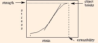
The graph of stress vs. strain for a material is a veritable cornucopia of information:
The slope of the curve at any point is called the Young's Modulus, and has dimensions of force over area.
Its numerical value is indicative of the stiffness of the material: smaller values indicate that less stress is required for more strain.
In general, the stress vs. strain curve will differ for each material, and for each type of stress.
The strength of the material is the maximum value of the stress before breakage.
The extensibility is the maximum value of the strain before breakage.
The toughness is the area under the curve between the vertical dashed lines, and is equal to the energy required to break the object.
The partial area under the curve up to a given strain (less than the extensibility) is the work of extension.
Hooke's Law is simply the linear part of the stress vs. strain graph.
The stress vs. strain curve is not necessarily the same during the relaxation of stress as it was during the loading (application) of the stress.
This phenomenon is called hysteresis, and the ratio of the area under the relaxation curve to that under the loading curve
(for a given strain) is called the resilience (usually expressed as a percentage).
With our knowledge of Hooke's Law we can now make the analogy between mechanical and electrical systems more precise.
In an
electrical circuit, charge
plays the same role as position does in mechanical systems; therefore current is analogous to velocity.
Since energy is voltage times charge, voltage must play the part of
mechanical force (since force is the gradient of energy). In fact,
electrical potential is often called electromotive force. We therefore have the following correspondences:
= - keffective (x1 + x2)
= - keffective (- F / k1 - F / k2)
The next section introduces us to waves, and discusses the effects of boundary conditions and superposition on standing waves.
©2009, Kenneth R. Koehler. All Rights Reserved. This document may be freely reproduced provided that this copyright notice is included.
Please send comments or suggestions to the author.
F = - k x
is called Hooke's Law. The spring constant clearly has units of force over distance, or kg / s2. Stiffer springs have larger spring constants; a moderately loose spring might have a spring constant of about 10 kg / s2.
U = k x2 / 2.
Small Oscillations
m a = - k x,
or
a = (-k / m) x.
In words, this means that the rate of change of the rate of change of position is proportional to the position. Graphically, we can try to picture the position as an oscillatory function of time: perhaps a sine function:
x(t) = sin (ω t)
or
x(t) = cos (ω t),
where
ω = (k / m)1/2.
In this case, we choose the cosine function, because at time t = 0 the mass was displaced a small distance from the origin; since sin (t) is zero at time zero, only the cosine can describe these oscillations.
k A2 / 2.
In fact, the position and velocity of this oscillator are
A cos (ω t) and
so that the sum of the kinetic and potential energies is
m (-A ω sin (ω t))2 / 2 +
k (A cos (ω t))2 / 2,
at every point along its trajectory.
= m ω2 A2 sin (ω t)2 / 2 +
k A2 cos (ω t)2 / 2
k x ± ω t ± δ.
δ is called the phase angle, and effectively allows us to specify the relative starting point of the oscillator at time zero. By experimenting with various values of δ (ie., 0, π/2, π, 3π/2, 2π), we see that we can produce oscillations which have any given initial value (between -A and A) at time zero.
. . .
 . . .
. . .
The first two correspondences would lead us to believe that the spring constant behaves like the inverse of the
capacitance.
However, consider a uniform mass suspended from the ceiling with two identical springs, one attached to each end of the mass.
In the mechanical system, both springs stretch the same displacement, and so we have
F = - k x V = Q / C U = k x2 / 2 U = Q2 / 2 C Fdrag = - b V V = I R
F = - k1 x - k2 x.
This means that two springs in parallel have an effective
spring constant which is simply the sum of the two spring constants.
If we connect the two springs in series (one on the end of the other)
and suspend our mass from the end, we have
F = - k1 x1
which means that the spring constants of springs in series behave like capacitances:
= - k2 x2
keffective = 1 / (1 / k1 + 1 / k2)
The lesson here is that isomorphisms can be useful tools,
but the relationships must reflect the physical phenomenology:
So the spring constant does behave like the inverse of the capacitance, but because the roles of charge and displacement,
voltage and force, behave oppositely in springs and capacitors, the equations for the effective spring constant of
springs in series and parallel are isomorphic to those for capacitance.
charge / displacement voltage / force capacitors in series same split between them springs in series split between them same capacitors in parallel split between them same springs in parallel same split between them